Your Mannequin’s MSE Is Mendacity to You

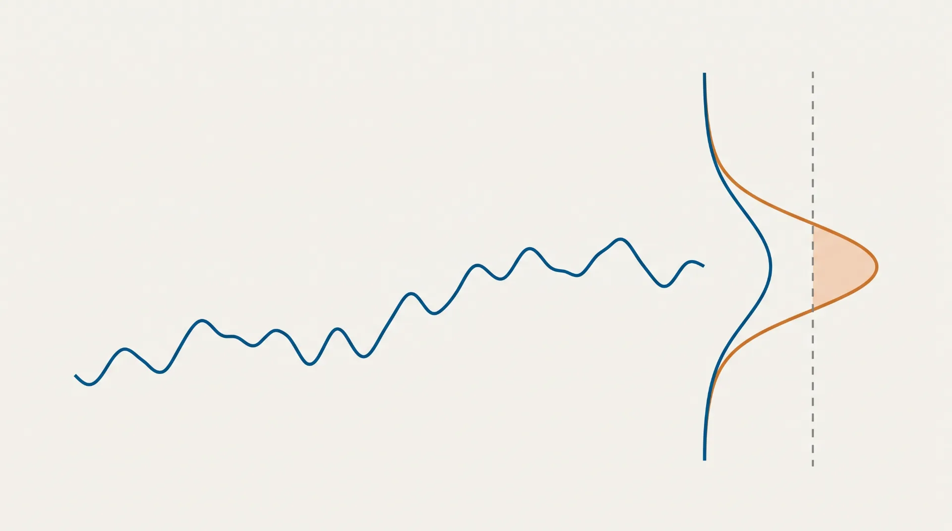
Two fashions, one quantity, reverse realities

Think about you might have a sensor recording one thing you care about, for instance seismic background at a detector web site, electrical load on a grid, or pressure in a bridge cable, and you’ve got skilled a mannequin to forecast the subsequent worth. The mannequin appears to be like on the latest historical past, thinks for a second, and offers you a single quantity: $0.5$.

There is a threshold $tau = 1.0$

You may’t reply that. Not since you’re lacking details about the mannequin, however as a result of the mannequin is lacking a technique to inform you what it is aware of. That single quantity $0.5$ is all it could possibly say. Let’s examine why that is an issue.

Think about you even have two fashions, each watching the identical sign, each predicting $hat{x} = 0.5$

This is what’s hiding beneath.

• Mannequin A is taking a look at a second the place the true conditional distribution, the precise unfold of values the sign may realistically take, given its latest historical past may be very tight:

  $x ;sim; mathcal{N}(0.5,; 0.01^{2})$

  If this notation is new to you: $mathcal{N}(mu, sigma^{2})$

• Mannequin B is taking a look at a second the place the true distribution is broad:

  $x ;sim; mathcal{N}(0.5,; 2.0^{2})$

  Similar middle, however $sigma = 2.0$

Similar forecast. Similar MSE. Similar check set. However the precise danger of triggering the alarm is $approx 0$

The issue is not that both mannequin is damaged. Each predicted the right imply. The issue is {that a} single quantity cannot specific I am positive versus I am guessing and the rationale the mannequin cannot specific that is not a coaching bug or a lacking characteristic. It is a direct, provable consequence of the loss operate it was skilled with.

That is what this submit unpacks. We’ll see precisely why MSE fingers you the imply and discards every little thing else, what to exchange it with, and what that substitute prices as soon as an actual optimizer will get maintain of it.

···

What forecasting truly asks

Let’s arrange the issue correctly, as a result of the belief we will break is hiding within the setup itself.

A time sequence is a sequence of numbers recorded so as over time.

For example, temperature each hour, inventory value at market shut every day, or displacement of a seismometer sampled at 100Hz. The important thing property is that the order carries info, the worth at time $t$ tells you one thing in regards to the worth at $t+1$

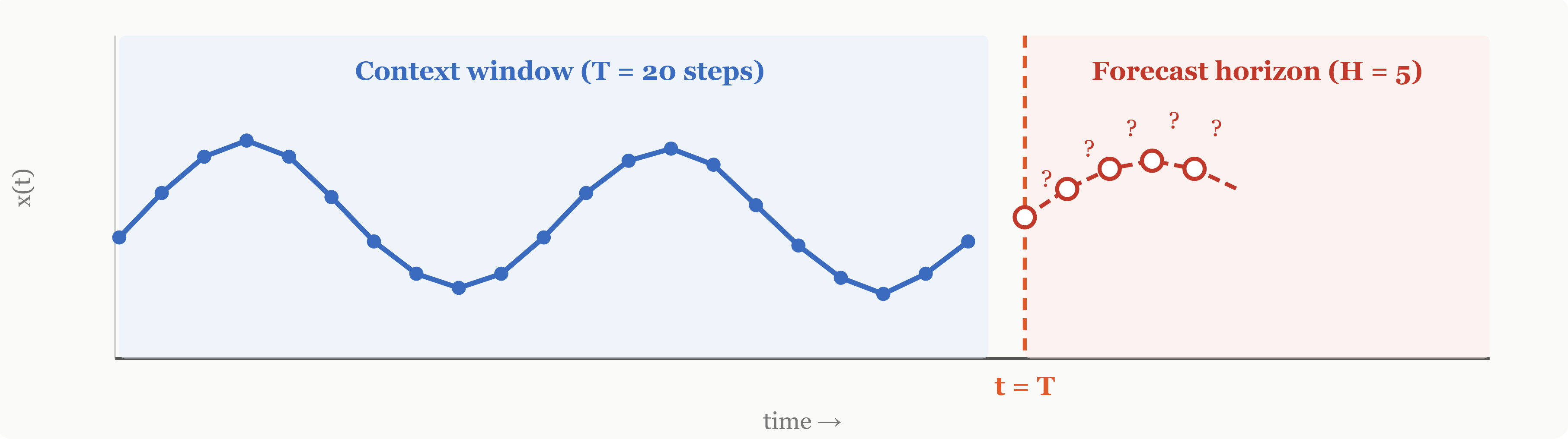
We write the noticed sequence as:

$x_{1},, x_{2},, ldots,, x_{T}$

the place $x_{t}$

$x_{T+1},, x_{T+2},, ldots,, x_{T+H}$

Two numbers management the setup:

• $T$= context size: how far again the mannequin appears to be like.

• $H$= forecast horizon: how far forward the mannequin predicts.

The best case is $H = 1$

Now here is the refined half that the majority textbooks gloss over. Whenever you write down your prediction as a single quantity $hat{x}_{T+1}$

Take into consideration what that single quantity means. The mannequin says the subsequent worth is 0.5, not most likely round 0.5, not someplace between 0.3 and 0.7, simply 0.5, full cease. That format has no room for doubt. There isn’t any subject within the output for by the way in which, I am undecided about this one.

No one agrees to this assumption on function. You conform to it by selecting a loss operate. The loss decides what the mannequin can and can’t specific, and the usual loss, MSE, decides for you: the reply is some extent, not a distribution.

···

The best loss, and what it truly optimizes

Probably the most pure factor a mannequin can do is emit one actual quantity $hat{x}_{T+h}$

$mathcal{L}_{mathrm{MSE}} ;=;frac{1}{N}sum_{i=1}^{N}bigl(x_{i} – hat{x}_{i}bigr)^{2}$

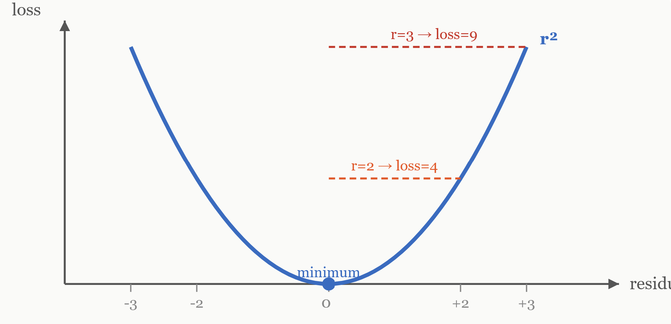
the place the sum runs over all coaching examples and timesteps. It is zero when the prediction is actual, and grows quadratically because the prediction drifts away:

• An error of two prices 4 instances an error of 1.

• An error of 10 prices 100 instances an error of 1.

Giant errors dominate the gradient, which is strictly what you need, miss the spike and you’ve got missed the purpose.

To this point, so good. The difficulty begins if you ask: what prediction does MSE truly reward? If the mannequin might be excellent, what would MSE push it towards?

The proof: with out historical past first

Let’s overlook about neural networks, architectures, every little thing. Simply pure math. Bear with me, the derivation is brief, and it tells you one thing basic.

You will have a random variable $x$, the subsequent worth the sign will take. You do not know what will probably be, nevertheless it has some distribution with imply $mu = mathbb{E}[x]$

We need to reduce:

$mathbb{E}bigl[(x – c)^{2}bigr]$

Broaden the sq. (simply $(a-b)^{2} = a^{2} – 2ab + b^{2}$

$mathbb{E}bigl[(x – c)^{2}bigr] ;=; mathbb{E}[x^{2}] ;-; 2c,mathbb{E}[x] ;+; c^{2}$

$mathbb{E}[x^{2}]$ is a set quantity (is determined by the distribution of $x$ , not our selection). $mathbb{E}[x]$ can also be mounted, that is $mu$. In order a operate of$c$ , it is a parabola opening upward. It has precisely one minimal.

Differentiate with respect to $c$ and set to zero:

$frac{d}{dc}Bigl[mathbb{E}[x^{2}] – 2c,mathbb{E}[x] + c^{2}Bigr];=; -2,mathbb{E}[x] + 2c ;=; 0$

 $boxed{c^{*} = mathbb{E}[x]}$

The optimum single-number prediction underneath squared error is the imply. Geometrically: the purpose closest on common, in squared distance, to a cloud of doable outcomes is the middle of that cloud.

Now with historical past

In forecasting, $x$ is not drawn from a set distribution. Its distribution is determined by the historical past, that’s, what the sign has been doing. Totally different pasts result in completely different futures. Now, write $mathcal{H} = (x_{1}, ldots, x_{T})$

$mathbb{E}bigl[(x – c)^{2} mid mathcal{H}bigr];=; mathbb{E}[x^{2} mid mathcal{H}] ;-; 2c,mathbb{E}[x mid mathcal{H}] ;+; c^{2}$

Differentiate with respect to $c$ , set to zero:

$-2,mathbb{E}[x mid mathcal{H}] + 2c = 0 quadLongrightarrowquad c^{*} = mathbb{E}bigl[x mid x_{1}, ldots, x_{T}bigr]$

Nothing modified structurally. The derivation is strictly the identical as earlier than, we simply added “$| mathcal{H}$” in all places.

That is what the MSE optimizes for:

$c^{*} = mathbb{E}bigl[x mid x_{1}, ldots, x_{T}bigr]$

The MSE-optimal prediction is the conditional imply. That is what any mannequin skilled with MSE is pushed towards, no matter structure (transformer, LSTM, linear regression, something). Given infinite knowledge and sufficient capability, the mannequin converges to predicting the common of the place the sign may go subsequent, given the previous it has seen.

The imply is a superbly affordable factor to foretell. No different single quantity does higher underneath squared error. However the imply is a single abstract of location. It tells you the place the middle of the distribution sits. Nonetheless, it tells you nothing about:

• Width: Is the distribution tight $sigma = 0.01$

• Form: Symmetric? Skewed? Heavy-tailed?

Two utterly completely different conditions can share an similar conditional imply and MSE, however by development, can’t inform them aside. It has no time period that rewards getting the width proper, and no time period that punishes getting it mistaken. The unfold is invisible to the loss. That is Mannequin A and Mannequin B restated within the language of the mathematics. Similar conditional imply, incompatible futures, one quantity.

···

The idea no one writes down

This is the place it will get worse. MSE would not merely ignore the unfold, ignoring it might be survivable. Coaching with it’s mathematically equal to assuming the unfold is the similar in all places. To see this, we want a brief detour by way of most probability estimation (MLE). Do not let the identify intimidate you, the concept is definitely fairly easy.

Most probability: the instinct

Neglect loss features for a second and give it some thought in a different way. Your mannequin, with parameters $theta$ , appears to be like on the historical past and makes a prediction. As a substitute of simply asking how shut was the prediction, ask a richer query: how possible did the mannequin assume the true end result was?.

Say the true worth turned out to be 3.7. A great mannequin ought to have thought 3.7 was doubtless. A foul mannequin thought 3.7 was a one-in-a-million occasion after which it occurred, which implies the mannequin had a nasty image of actuality.

Most probability simply says: choose the mannequin parameters $theta$ that make the noticed knowledge as possible as doable. The settings underneath which actuality appears to be like least stunning. However to assign possibilities to outcomes, we want a noise mannequin, an assumption about how noticed values scatter across the prediction. Probably the most pure start line is a Gaussian with some mounted width.

The noise assumption

Assume that what you observe equals the mannequin’s prediction plus random noise:

$x = hat{x} + varepsilon, qquad varepsilon sim mathcal{N}(0,, sigma^{2})$

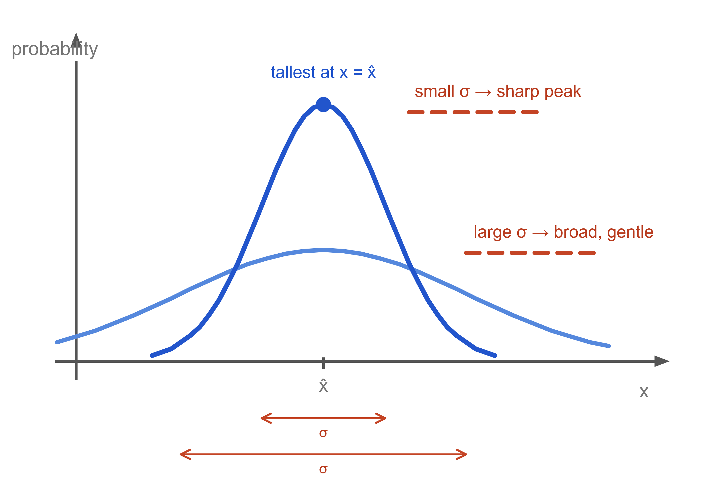
In phrases: the true worth is the prediction, plus a small random perturbation drawn from a Gaussian centered at zero with variance $sigma^{2}$ . The important thing phrase right here is mounted, the identical $sigma^{2}$ for each knowledge level, each timestep, each enter. Underneath this assumption, the chance density of observing $x$ given the prediction $hat{x}$

$p(x mid hat{x}) ;=; frac{1}{sqrt{2pisigma^{2}}}, exp!Biggl(-frac{(x – hat{x})^{2}}{2sigma^{2}}Biggr)$

If this method is new to you: it is tallest when $x = hat{x}$

From chance to loss operate

Now you might have $N$ unbiased observations. Each has a chance underneath the mannequin. The overall chance of all the dataset is the product:

$mathcal{L} = prod_{i=1}^{N} p(x_{i} mid hat{x}_{i})$

Merchandise of many small numbers underflow to zero on a pc, and their derivatives are messy. So we take the logarithm. Since $log$ is monotonically growing, the parameters that maximize the product additionally maximize the logarithm. The product turns into a sum:

$log mathcal{L} ;=; sum_{i=1}^{N} log, p(x_{i} mid hat{x}_{i})$

Plug within the Gaussian density. For a single time period:

$log, p(x_{i} mid hat{x}_{i}) ;=; log!biggl(frac{1}{sqrt{2pisigma^{2}}}biggr) ;-; frac{(x_{i} – hat{x}_{i})^{2}}{2sigma^{2}}$

The primary half is $-tfrac{1}{2}log(2pisigma^{2})$

$log mathcal{L} ;=; -frac{N}{2}log(2pisigma^{2}) ;-; frac{1}{2sigma^{2}}sum_{i=1}^{N}(x_{i} – hat{x}_{i})^{2}$

Now, maximize over the predictions $hat{x}_{i}$

• First time period: $-tfrac{N}{2}log(2pisigma^{2})$

• Second time period: $-tfrac{1}{2sigma^{2}}sum_{i}(x_{i} – hat{x}_{i})^{2}$

Strip each away, and maximizing the log-likelihood is exactly minimizing:

$sum_{i=1}^{N}(x_{i} – hat{x}_{i})^{2}$

That is MSE. Now learn it backwards.

Each time you practice with MSE, you might have implicitly assumed that the residuals $(x_{i} – hat{x}_{i})$

And as soon as coaching ends, even that single $sigma$ is gone. It lived solely contained in the derivation. The skilled mannequin fingers you $hat{x}$

Why fixed variance is sort of all the time mistaken

Take into consideration what fixed $sigma$ means in follow. The mannequin is pressured to be equally assured in all places:

• Forecasting electrical energy demand on an peculiar Tuesday night time: simple, low variance. Forecasting it throughout a shock heatwave: onerous, excessive variance. Similar $sigma$for each? That is the belief.

• Seismic background at a detector web site on a quiet day: nearly flat, very predictable. Throughout a teleseismic occasion: wild fluctuations. Similar $sigma$for each? That is the belief.

The technical time period for fixed variance is homoscedastic. Nonetheless, in a practical scenario, variance that adjustments with the enter is heteroscedastic. Virtually each actual bodily and financial sign is heteroscedastic. MSE cannot symbolize that.

That is precisely what separated Mannequin A from Mannequin B mentioned above. The true conditional variance was $0.01^{2}$ in a single case and $2.0^{2}$ within the different. An MSE-trained mannequin suits one $sigma$ for the entire dataset and applies it in all places, too broad when issues are calm, too slim when issues are unstable, mistaken in each instructions. That is the crack within the basis, however, the repair is shorter than you’d assume.

···

The leap: predict a distribution

The entire drawback comes down to at least one factor: $sigma$ by no means seems within the mannequin’s output. It was hiding contained in the derivation that produced MSE, it was mounted to at least one worth for all the dataset, and it vanished after coaching. The mannequin actually has no technique to say I am unsure right here.

The repair may be very easy. As a substitute of emitting a single quantity, make the mannequin emit the parameters of a chance distribution.

The best selection, and the pure one, on condition that MSE was already implicitly Gaussian, is 2 numbers:

$(mu,; sigma) ;=; f_{theta}(x_{1}, ldots, x_{T})$

the place $mu$ is the anticipated middle and $sigma > 0$

$x_{T+1} ;sim; mathcal{N}(mu,; sigma^{2})$

In phrases: I believe the subsequent worth is drawn from a bell curve centered at $mu$ with customary deviation$sigma$.

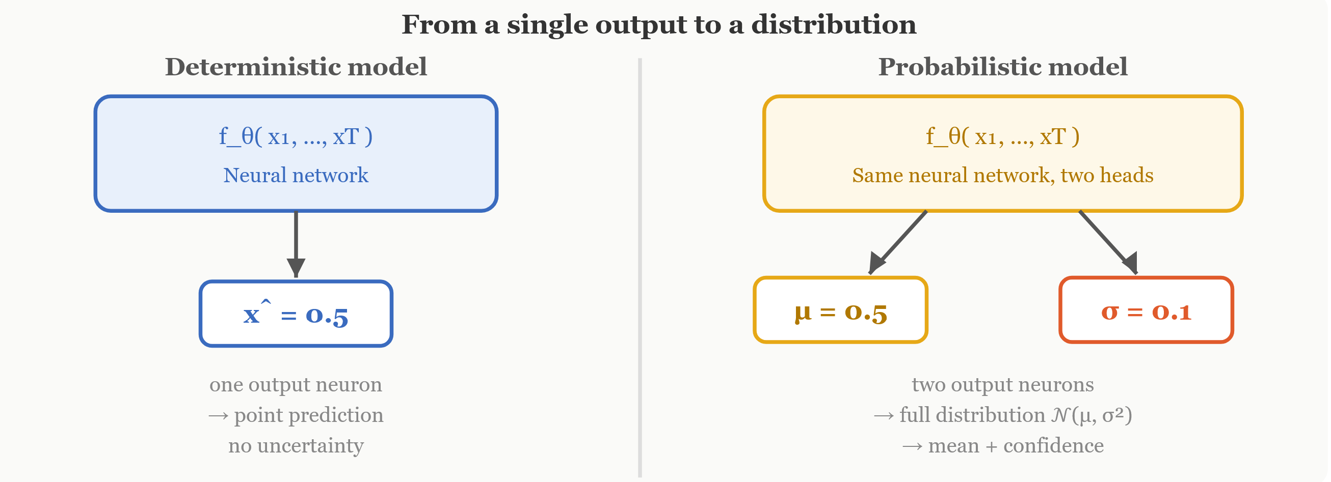
That could be a greater change than one further output neuron suggests. The output area adjustments from $R$ (a single level on the quantity line) to a distribution over $R$. The mannequin stops committing to at least one reply and begins reporting a weighted vary of prospects, together with how broad that vary needs to be at this explicit second, given this explicit historical past.

And $sigma$ is now not a single international quantity. It is a operate of the enter. The identical mannequin can output $sigma = 0.01$

Architecturally, the change is minimal. The spine, each consideration head, each hidden layer, all of the characteristic extraction, stays similar. The ultimate layer positive factors one further output neuron. One neuron produces $mu$, the opposite produces $sigma$. That is it. However now we want a brand new loss. MSE solely is aware of evaluate one quantity to at least one quantity, it has no thought what to do with $sigma$. When you practice with MSE, the $mu$ head will study (MSE can rating it), however the $sigma$ head will get no gradient sign in any respect. We want one thing that trains each.

···

Asking a greater query

Your mannequin predicts that the subsequent worth follows:

$y ;sim; mathcal{N}bigl(mu_{theta}(mathbf{x}),;; sigma_{theta}^{2}(mathbf{x})bigr)$

Then the true worth $y$ is revealed. How will we rating the prediction?

Neglect formulation for a second. Give it some thought intuitively. The mannequin drew a bell curve. That bell curve assigns a chance density to each doable end result, excessive density close to the middle, low density out within the tails.

Then actuality handed us a particular quantity $y$. If $y$ landed close to the height, the place the mannequin put plenty of chance, the mannequin did properly. It thought this end result was doubtless, and it was proper. If $y$ landed means out within the tails, the place the mannequin put nearly no chance, the mannequin did poorly. It was stunned by actuality. So the pure rating is: how a lot chance density did the mannequin assign to the worth that really occurred?

That density is:

$p_{theta}(y mid mathbf{x}) ;=; frac{1}{sqrt{2pisigma_{theta}^{2}}}, exp!biggl(-frac{(y – mu_{theta})^{2}}{2sigma_{theta}^{2}}biggr)$

We would like this to be giant. Since $-log$ is monotonically lowering, maximizing this density is similar as minimizing the unfavourable log-likelihood:

$mathcal{L}(y,, mu_{theta},, sigma_{theta}) ;=; -log, p_{theta}(y mid mathbf{x})$

Why the logarithm? Two causes. Virtually: coaching minimizes losses, so we negate to flip maximize into reduce. As well as, numerically: likelihoods over many knowledge factors are merchandise of small numbers (which underflow); $log$ turns merchandise into sums, conserving issues steady. Discover the shift in philosophy:

• MSE asks: How far was your quantity from the reality?

• NLL asks: How stunned ought to you might have been by the reality, given the distribution you predicted?

The second query is richer as a result of it includes each the middle and the width.

Now let’s derive the method. No methods, simply algebra. Bear with me, it is simply 4 traces after which we’re performed. Begin from the Gaussian density:

$p(y mid mu, sigma) ;=; frac{1}{sqrt{2pisigma^{2}}}, exp!biggl(-frac{(y-mu)^{2}}{2sigma^{2}}biggr)$

Step 1: take the logarithm: The expression is a product (fraction instances exponential), so $log$ splits it right into a sum:

$log p(y mid mu, sigma) ;=; log!biggl(frac{1}{sqrt{2pisigma^{2}}}biggr) ;-; frac{(y – mu)^{2}}{2sigma^{2}}$

Step 2: broaden the primary time period. Utilizing $log(1/a) = -log a$

$log!biggl(frac{1}{sqrt{2pisigma^{2}}}biggr) ;=; -tfrac{1}{2}log(2pi) ;-; tfrac{1}{2}log(sigma^{2}) ;=; -tfrac{1}{2}log(2pi) ;-; log(sigma)$

Step3: assemble.

$log p(y mid mu, sigma) ;=; -tfrac{1}{2}log(2pi) ;-; log(sigma) ;-; frac{(y – mu)^{2}}{2sigma^{2}}$

Step 4: negate and drop the fixed. The time period $tfrac{1}{2}log(2pi) approx 0.919$

$boxed{mathcal{L}_{mathrm{Gauss}}(y,,mu,,sigma) ;=; underbrace{frac{(y-mu)^{2}}{2sigma^{2}}}_{textual content{match time period}};+; underbrace{log(sigma)}_{textual content{honesty time period}}}$

Two phrases, two jobs. They usually do not cooperate, they battle. The battle is the mechanism.

···

Two phrases and the battle between them

Understanding this competitors is the important thing to understanding each failure mode you will probably meet later. Let’s take the 2 phrases one by one.

The match time period: $(y – mu)^{2},/,2sigma^{2}$

The numerator is the squared residual, precisely MSE. The brand new aspect is the denominator: $2sigma^{2}$, which is the mannequin’s claimed variance (instances 2).

Dividing by $sigma^{2}$makes the penalty relative to the arrogance the mannequin claimed earlier than seeing the reply.

Think about the mannequin predicted $mu = 0.5$

• $sigma = 0.1$

• $sigma = 1.0$

• $sigma = 10.0$

The mannequin is allowed to make errors, however provided that it admitted beforehand that these errors had been doable. The worth of $sigma$was chosen earlier than $y$ was revealed, no dishonest after the actual fact. However here is the catch. The match time period will get cheaper as $sigma$ grows. At all times. For any mounted residual, an even bigger $sigma$means a smaller penalty. So if this had been the one time period, the mannequin would uncover a trivial technique: set $sigma = infty$

The honesty time period:$logsigma$

This closes that door.$logsigma$ will increase as $sigma$ will increase. That is it. That is the entire mechanism.

• Small $sigma$ (excessive confidence): $logsigma$ is small and even unfavourable. This reduces the full loss. The mannequin is rewarded for precision.

• Giant $sigma$ (low confidence): $logsigma$ is giant and optimistic. This will increase the full loss. The mannequin pays a value for hedging.

The stability

Put each phrases collectively:

$mathcal{L} ;=; frac{(y – mu)^{2}}{2sigma^{2}} ;+; log(sigma)$

The match time period says: make $sigma$ greater so my errors value much less, whereas the honesty time period says: make $sigma$ smaller so I get rewarded for precision. These two forces pull in reverse instructions, and the mannequin has to search out the place they stability. That stability will not be a hand-tuned tradeoff. There isn’t any hyperparameter weighting the 2 phrases, they got here from the identical derivation, from the identical logarithm of the identical Gaussian density. The stability falls out of the mathematics.

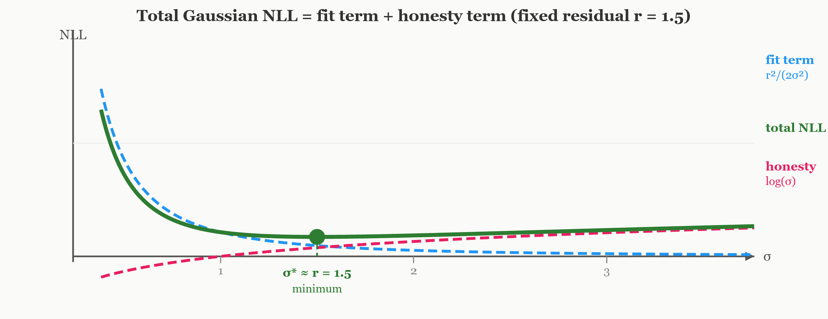
To make this concrete, repair the residual at $r = y – mu = 1.5$

The minimal is at $sigma approx 1.5$

Wow, that is not a coincidence. The following part proves it precisely.

···

What the optimum needs to be

We have seen the instinct. Now let’s discover the stability precisely.

Optimum $mu^{*}$

Maintain $sigma$ mounted and optimize $mu$. The one $mu$-dependent a part of the loss is:

$mathbb{E}_{y}!biggl[frac{(y-mu)^{2}}{2sigma^{2}}biggr] ;=; frac{1}{2sigma^{2}};mathbb{E}_{y}!bigl[(y-mu)^{2}bigr]$

That is MSE multiplied by the optimistic fixed $tfrac{1}{2sigma^{2}}$

$boxed{mu^{*} = mathbb{E}[y mid mathcal{x}]}$

NLL and MSE agree utterly on the place the middle needs to be. The $sigma$ within the denominator rescales the penalty however would not shift the optimum. All the things the mannequin already knew do is preserved.

Optimum $sigma^{*}$

Now repair $mu = mu^{*}$

$v ;=; mathbb{E}bigl[(y – mu^{*})^{2} mid mathbb{x}bigr]$

That is how unfold out $y$ truly is round its imply, given the enter. It is a property of the info, not the mannequin. From $sigma$‘s perspective, $v$ is only a mounted optimistic quantity.

The anticipated loss as a operate of $sigma$:

$f(sigma) ;=; frac{v}{2sigma^{2}} ;+; log(sigma)$

Differentiate. The by-product of $tfrac{v}{2}sigma^{-2}$

The by-product of $logsigma$ is $tfrac{1}{sigma}$

$frac{df}{dsigma} ;=; -frac{v}{sigma^{3}} ;+; frac{1}{sigma} ;=; 0$

$frac{1}{sigma} = frac{v}{sigma^{3}} qquadLongrightarrowqquad sigma^{2} = v$

$boxed{sigma^{*2} ;=; mathbb{E}bigl[(y – mu^{*})^{2} mid mathbb{x}bigr] ;=; mathrm{Var}(y mid mathbb{x})}$

Gaussian NLL pushes $sigma^{2}$ towards the true conditional variance.

The mannequin learns each the conditional imply and the conditional variance concurrently, one loss operate, two targets.

This implies the uncertainty will not be a manually chosen fixed. The mannequin produces a special $sigma$ for each enter, matching the precise native noise. When the sign is in a relaxed regime, $mathrm{Var}(y mid mathbb{x})$

That is the lacking piece from Sections 1-4. Mannequin A’s small variance $0.01^{2}$) and Mannequin B’s giant variance ($2.0^{2}$) can lastly be distinguished, as a result of the loss provides the mannequin a cause to study them.

···

Why that is the appropriate loss, not merely an excellent one

All the things to this point has been: here is a loss, the mathematics works out, the optimum is good. However you possibly can moderately ask why this loss? Might you cook dinner up a special two-term penalty that additionally balances $mu$ and $sigma$? One thing like $textual content{MSE} + lambda cdot sigma^{2}$

Certainly, that will additionally penalize giant $sigma$. It would even work okay. However it might be an arbitrary recipe with no principled interpretation. Gaussian NLL is not one recipe amongst many. It has a deeper justification from info concept.

KL divergence: the instinct

Let $p_{mathrm{true}}(y mid mathbb{x})$

In the event that they match completely, KL is strictly zero, no info misplaced. The extra they differ, the bigger the KL. The KL divergence is outlined as:

$D_{mathrm{KL}}!bigl(p_{mathrm{true}} ,|, p_{theta}bigr) ;=; mathbb{E}_{p_{mathrm{true}}}!biggl[log frac{p_{mathrm{true}}(y)}{p_{theta}(y)}biggr]$

Broaden the log ratio:

$=; mathbb{E}_{p_{mathrm{true}}}!bigl[log p_{mathrm{true}}(y)bigr] ;-; mathbb{E}_{p_{mathrm{true}}}!bigl[log p_{theta}(y)bigr]$

The primary time period is the unfavourable entropy of the true distribution, it is a mounted quantity that relies upon solely on floor fact (actuality), not on the mannequin. From $theta$‘s perspective, it is a fixed. The second time period is the anticipated log-likelihood underneath the mannequin. So:

$D_{mathrm{KL}}!bigl(p_{mathrm{true}} ,|, p_{theta}bigr) ;=; mathbb{E}_{p_{mathrm{true}}}!bigl[,underbrace{-log p_{theta}(y)}_{text{NLL}},bigr] ;+; textual content{const}$

The deep connection

$textbf{Minimizing anticipated NLL} ;=; textbf{Minimizing } D_{mathrm{KL}}(p_{mathrm{true}} ,|, p_{theta})$

Whenever you reduce NLL, you might be minimizing the information-theoretic distance between the mannequin’s predicted distribution and the bottom fact. You are dragging $p_{theta}$

As well as, KL divergence would not simply care in regards to the imply or the variance. It cares about each facet of the distribution, resembling skewness, kurtosis, tail habits, every little thing. The one cause we study simply imply and variance right here is that we selected a Gaussian for $p_{theta}$

The cleanest technique to see the basic distinction:

• MSE minimizes a distance between two numbers.

• NLL minimizes a distance between two distributions.

MSE operates within the area of values. NLL operates within the area of chance distributions. The second is infinitely richer. And here is the attractive half: if you limit NLL to a Gaussian with mounted $sigma$, it collapses again to MSE, that was Part 4. MSE is a particular case of NLL, the case the place you have given up on studying uncertainty. NLL is the final framework; MSE is what you get if you freeze $sigma$ and throw it away.

···

Sensible Engineering

Stunning goal. Now make it survive when it really works with an optimizer. To attain this, two engineering particulars have to be taken into consideration and one deeper difficulty stands between the derivation and the code that trains.

Predict $logsigma$, not $sigma$

The output layer produces any actual quantity, however $sigma$ have to be strictly optimistic. How do you implement that?

• ReLU: $sigma = max(0, h)$

• Softplus: $sigma = log(1 + e^{h})$

• The usual transfer: let the community predict $s = logsigma$

$mathcal{L}_{mathrm{Gauss}} ;=; frac{(y – mu)^{2}}{2e^{2s}} ;+; s$

Each $mu$ and $s$ now vary freely over $R$. Nothing for the optimizer to battle.

Clamp the vary

Even reparameterized, $s$ can wander someplace ineffective:

• $s to -infty$

• $s to +infty$

A easy clamp retains issues sane:

log_sigma = torch.clamp(log_sigma, min=-6.0, max=2.0)sigma     = torch.exp(log_sigma)

This provides $sigma in [e^{-6}, e^{2}] approx [0.0025,, 7.4]$

The optimization lure

This one is subtler. It is not about numerical stability, it is in regards to the optimization panorama. Have a look at the gradient of the match time period with respect to $mu$:

$frac{partial}{partialmu}biggl[frac{(y-mu)^{2}}{2sigma^{2}}biggr] ;=; -,frac{y – mu}{sigma^{2}}$

See the $1/sigma^{2}$? The gradient that updates $mu$ is scaled by the inverse of $sigma^{2}$. When $sigma$ is properly calibrated, that is tremendous. However early in coaching, here is what occurs:

• The mannequin begins with random parameters. Predictions are dangerous, giant residuals in all places.

• Two paths to scale back the loss: enhance $mu$ (onerous, requires studying sign construction) or enhance $sigma$ (simple, simply shift the $s$ output upward).

• The mannequin takes the simple path, $sigma$ grows.

• As $sigma$ grows, the $1/sigma^{2}$ issue shrinks. The gradient on $mu$ weakens.

• The mannequin stops enhancing $mu$ for the onerous examples, as a result of it already labeled them as unsure.

A vicious cycle: giant $sigma$ $to$ weak $mu$-gradient $to$ $mu$ stays dangerous $to$ giant residuals justify giant $sigma$. The mannequin learns to clarify away its personal errors by claiming uncertainty, as an alternative of truly getting higher. And the examples the place this occurs most are precisely the toughest ones, those the mannequin most must study from.

There are two sensible fixes:

• MSE warmup. Practice with plain MSE first, ignoring the $sigma$ head. As soon as $mu$ in all fairness correct, swap to NLL. Now $sigma$ has a significant sign to study from, and the shortcut of inflating $sigma$ is much less tempting as a result of the predictions aren’t that dangerous anymore.

• $beta$-NLL. Multiply every pattern’s loss by a indifferent issue of $sigma^{2beta}$.

This reweights gradients so onerous examples preserve contributing even when $sigma$ is giant. At $beta = 0$

The important thing lesson: a loss operate can have a mathematically appropriate optimum and nonetheless be troublesome to optimize in follow. Proving that $sigma^{*2} = mathrm{Var}(y mid mathbb{x})$

···

The place the pocket book picks up

All the things above is the derivation. Now the query we parked: does this truly occur if you practice an actual mannequin?

The companion notebook builds two transformers with the identical spine, on the identical artificial sign. The sign is designed in order that its noise stage adjustments over time, quiet stretches and noisy stretches, and no one tells both mannequin the place the boundaries are.

• Mannequin 1: skilled with MSE. Outputs one quantity per timestep.

• Model2: skilled with Gaussian NLL. Outputs $mu$ and $sigma$.

On plain level accuracy, they end almost comparable. We already predicted this: NLL and MSE agree on the optimum $mu$, so including $sigma$ would not damage level predictions. On this metric alone, you’d name them interchangeable. However they don’t seem to be. Cut up the check set into quiet and noisy regimes. Ask every mannequin to attract a 90% prediction interval, a band that ought to comprise the true worth 90% of the time. For the level mannequin, the one choice is one mounted band width computed from the worldwide residual variance. For the probabilistic mannequin, every timestep has its personal $sigma$, so the band is $mu pm 1.645sigma$

The purpose mannequin overshoots the 90% goal when issues are calm (the mounted band is simply too broad) and catastrophically undershoots when issues are noisy (the band is way too slim). One in three values that needs to be contained in the interval falls outdoors. The probabilistic mannequin stays roughly trustworthy in each regimes, as a result of its band truly tracks the native noise. Proper on common, mistaken the place it issues. That is the entire argument in a single desk.

The pocket book additionally closes the circle on the brink query from the opening. Given a threshold, the purpose predictor can solely say sure or no. The probabilistic mannequin returns an actual chance, the amount a choice truly wants. And there’s a plot of the anticipated $sigma$ widening and narrowing with the true noise. The mannequin discovered that from the knowledge, as a result of the loss gave it a cause to.

···

Conclusion

MSE will not be a nasty loss operate. It does an excellent job of studying the middle of the goal distribution. But it surely says nothing in regards to the uncertainty. $sigma$ by no means seems within the MSE method. If the loss by no means sees uncertainty, it can’t study it or consider it. That’s, coaching with MSE implicitly assumes that the identical quantity of uncertainty applies in all places, an assumption that’s hardly ever true in real-world knowledge.

Gaussian NLL fixes this by letting the mannequin predict each $mu$ and $sigma$. The loss has two competing components: one encourages the mannequin to elucidate the info precisely, the opposite discourages it from claiming pointless uncertainty. Collectively, these forces drive the mannequin towards the true conditional variance. By means of the KL divergence connection, this goal is not a handy heuristic, it minimizes the information-theoretic hole between the mannequin’s distribution and actuality’s. With one further output neuron and a easy clamp, the mannequin learns each the imply and the uncertainty in a single coaching run.

Two necessary classes to hold ahead:

• First, predicted uncertainty is simply as dependable because the optimization course of that produced it. Though Gaussian NLL has an accurate optimum, coaching would not all the time attain it. The $1/sigma^{2}$ weighting creates a shortcut that may lure early studying. Sensible strategies, resembling MSE warmup and $beta$-NLL, make the trail to the optimum extra dependable.

• Second, the Gaussian continues to be an assumption. Predicting $sigma$ provides the mannequin an input-dependent measure of uncertainty, however the predicted distribution stays unimodal (one peak) and symmetric (equal chance above and beneath the imply). Some issues do not match this form. Think about a ball balanced on a ridge: it may roll left or proper, and the imply (the ridge prime) is the one place it will not keep. Knowledge with a number of doable futures, sudden regime adjustments, or heavy tails requires richer predictive distributions than a single Gaussian can present.

That’s the place extra expressive approaches, resembling quantized-token fashions and circulate matching, grow to be helpful, and the place the subsequent a part of this sequence begins. Till then, assume again to the query we began with: Ought to I fear about this prediction? A mannequin skilled solely with MSE has no significant technique to reply. A probabilistic mannequin skilled with Gaussian NLL lastly can.

···

References

[1] D. A. Nix and A. S. Weigend, Estimating the imply and variance of the goal chance distribution, Proc. IEEE Worldwide Convention on Neural Networks, 1994.

[2] A. Kendall and Y. Gal, What Uncertainties Do We Want in Bayesian Deep Studying for Pc Imaginative and prescient?, Advances in Neural Data Processing Programs (NeurIPS), 2017.

[3] T. Gneiting and M. Katzfuss, Probabilistic Forecasting, Annual Evaluation of Statistics and Its Utility, 2014.

[4] M. Seitzer, A. Tesch, N. Rasiwasia, and G. Martius, On the Pitfalls of Heteroscedastic Uncertainty Estimation with Probabilistic Neural Networks, ICLR 2022.