


Massive language fashions encompass billions of parameters (weights). The mannequin should carry out computationally intensive calculations throughout all of those parameters for every phrase it generates.
A big-scale language mannequin accepts a sequence of sentences or tokens after which generates a chance distribution of doubtless tokens.
So usually you’ll decode n token (or technology) n mannequin phrase) requires operating the mannequin n Variety of instances. At every iteration, new tokens are added to the enter sentence and handed to the mannequin once more. This may be pricey.
Moreover, the decoding technique can have an effect on the standard of the phrases produced. Producing tokens just by taking the token with the best chance within the output distribution can lead to textual content showing repeatedly. Random sampling from a distribution can introduce unintended drift.
Subsequently, a strong decoding technique is required to make sure each:
- Prime quality output
- Quick inference time
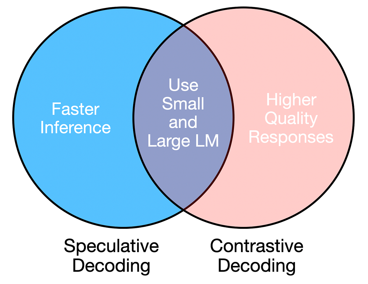
So long as the newbie and professional fashions are related (e.g. have the identical structure however completely different sizes), a mix of huge and small language fashions can tackle each necessities. Masu.
- Goal/Massive Mannequin: Essential LM with extra parameters (e.g. OPT-13B)
- Newbie/Petite Mannequin: A smaller model of the primary LM with fewer parameters (e.g. OPT-125M)
speculative and contrasting Decoding makes use of massive and small LLMs to realize dependable and environment friendly textual content technology.

Contrastive decoding This technique takes benefit of the truth that failures in massive LLMs (repetition, inconsistency, and so on.) are much more pronounced in small LLMs. Subsequently, this technique optimizes the tokens with the best chance distinction between the small and enormous fashions.
For one prediction, distinction decoding produces two chance distributions.
- q = Newbie mannequin logit chance
- p = Skilled mannequin logit chance
The subsequent token is chosen based mostly on the next standards:
- Discard all tokens whose chance just isn’t excessive sufficient underneath the professional mannequin (discard) p(x) < alpha * max(p))
- From the remaining tokens, select the one with the most important distinction in log chance between the big and small fashions. max(p(x) – q(x)).

Implementing contrastive decoding
from transformers import AutoTokenizer, AutoModelForCausalLM
import torch# Load fashions and tokenizer
tokenizer = AutoTokenizer.from_pretrained('gpt2')
amateur_lm = AutoModelForCausalLM.from_pretrained('gpt2')
expert_lm = AutoModelForCausalLM.from_pretrained('gpt2-large')
def contrastive_decoding(immediate, max_length=50):
input_ids = tokenizer(immediate, return_tensors="pt").input_ids
whereas input_ids.form[1] < max_length:
# Generate newbie mannequin output
amateur_outputs = amateur_lm(input_ids, return_dict=True)
amateur_logits = torch.softmax(amateur_outputs.logits[:, -1, :], dim=-1)
log_probs_amateur = torch.log(amateur_logits)
# Generate professional mannequin output
expert_outputs = expert_lm(input_ids, return_dict=True)
expert_logits = torch.softmax(expert_outputs.logits[:, -1, :], dim=-1)
log_probs_exp = torch.log(expert_logits)
log_probs_diff = log_probs_exp - log_probs_amateur
# Set an alpha threshold to get rid of much less assured tokens in professional
alpha = 0.1
candidate_exp_prob = torch.max(expert_logits)
# Masks tokens under threshold for professional mannequin
V_head = expert_logits < alpha * candidate_exp_prob
# Choose the following token from the log-probabilities distinction, ignoring masked values
token = torch.argmax(log_probs_diff.masked_fill(V_head, -torch.inf)).unsqueeze(0)
# Append token and accumulate generated textual content
input_ids = torch.cat([input_ids, token.unsqueeze(1)], dim=-1)
return tokenizer.batch_decode(input_ids)
immediate = "Massive Language Fashions are"
generated_text = contrastive_decoding(immediate, max_length=25)
print(generated_text)
speculative decoding That is based mostly on the precept that smaller fashions ought to pattern from the identical distribution as bigger fashions. Subsequently, this technique goals to simply accept as many predictions from the smaller mannequin as potential, so long as they match the distribution of the bigger mannequin.
The smaller mannequin produces n Place the tokens so as as potential guesses. Nonetheless, all n Sequences are fed into a big professional mannequin as a single batch, which is quicker than sequential technology.
This creates a cache for every mannequin. n Chance distribution inside every cache.
- q = Newbie mannequin logit chance
- p = Skilled mannequin logit chance
The tokens sampled from the newbie mannequin are then accepted or rejected based mostly on the next situations:
- If the chance of a token is increased within the professional distribution (p) than within the newbie distribution (q), or p(x) > q(x), settle for token
- If the chance of a token is decrease within the professional distribution (p) than within the newbie distribution (q), or p(x) < q(x)reject the token with chance 1 – p(x) / q(x)
If a token is rejected, the following token is sampled from the professional or adjusted distribution. Moreover, newbie and professional fashions reset and regenerate their caches. n Guessing and chance distributions p and q.

Implementing speculative decoding
from transformers import AutoTokenizer, AutoModelForCausalLM
import torch# Load fashions and tokenizer
tokenizer = AutoTokenizer.from_pretrained('gpt2')
amateur_lm = AutoModelForCausalLM.from_pretrained('gpt2')
expert_lm = AutoModelForCausalLM.from_pretrained('gpt2-large')
# Pattern subsequent token from output distribution
def sample_from_distribution(logits):
sampled_index = torch.multinomial(logits, 1)
return sampled_index
def generate_cache(input_ids, n_tokens):
# Retailer logits at every step for newbie and professional fashions
amateur_logits_per_step = []
generated_tokens = []
batch_input_ids = []
with torch.no_grad():
for _ in vary(n_tokens):
# Generate newbie mannequin output
amateur_outputs = amateur_lm(input_ids, return_dict=True)
amateur_logits = torch.softmax(amateur_outputs.logits[:, -1, :], dim=-1)
amateur_logits_per_step.append(amateur_logits)
# Sampling from newbie logits
next_token = sample_from_distribution(amateur_logits)
generated_tokens.append(next_token)
# Append to input_ids for subsequent technology step
input_ids = torch.cat([input_ids, next_token], dim=-1)
batch_input_ids.append(input_ids.squeeze(0))
# Feed IDs to professional mannequin as batch
batched_input_ids = torch.nn.utils.rnn.pad_sequence(batch_input_ids, batch_first=True, padding_value=0 )
expert_outputs = expert_lm(batched_input_ids, return_dict=True)
expert_logits = torch.softmax(expert_outputs.logits[:, -1, :], dim=-1)
return amateur_logits_per_step, expert_logits, torch.cat(generated_tokens, dim=-1)
def speculative_decoding(immediate, n_tokens=5, max_length=50):
input_ids = tokenizer(immediate, return_tensors="pt").input_ids
whereas input_ids.form[1] < max_length:
amateur_logits_per_step, expert_logits, generated_ids = generate_cache(
input_ids, n_tokens
)
accepted = 0
for n in vary(n_tokens):
token = generated_ids[:, n][0]
r = torch.rand(1).merchandise()
# Extract possibilities
p_x = expert_logits[n][token].merchandise()
q_x = amateur_logits_per_step[n][0][token].merchandise()
# Speculative decoding acceptance criterion
if ((q_x > p_x) and (r > (1 - p_x / q_x))):
break # Reject token and restart the loop
else:
accepted += 1
# Verify size
if (input_ids.form[1] + accepted) >= max_length:
return tokenizer.batch_decode(input_ids)
input_ids = torch.cat([input_ids, generated_ids[:, :accepted]], dim=-1)
if accepted < n_tokens:
diff = expert_logits[accepted] - amateur_logits_per_step[accepted][0]
clipped_diff = torch.clamp(diff, min=0)
# Pattern a token from the adjusted professional distribution
normalized_result = clipped_diff / torch.sum(clipped_diff, dim=0, keepdim=True)
next_token = sample_from_distribution(normalized_result)
input_ids = torch.cat([input_ids, next_token.unsqueeze(1)], dim=-1)
else:
# Pattern immediately from the professional logits for the final accepted token
next_token = sample_from_distribution(expert_logits[-1])
input_ids = torch.cat([input_ids, next_token.unsqueeze(1)], dim=-1)
return tokenizer.batch_decode(input_ids)
# Instance utilization
immediate = "Massive Language fashions are"
generated_text = speculative_decoding(immediate, n_tokens=3, max_length=25)
print(generated_text)
analysis
Each decoding approaches may be evaluated by evaluating them to a easy decoding methodology that randomly selects the following token from a chance distribution.
def sequential_sampling(immediate, max_length=50):
"""
Carry out sequential sampling with the given mannequin.
"""
# Tokenize the enter immediate
input_ids = tokenizer(immediate, return_tensors="pt").input_idswith torch.no_grad():
whereas input_ids.form[1] < max_length:
# Pattern from the mannequin output logits for the final token
outputs = expert_lm(input_ids, return_dict=True)
logits = outputs.logits[:, -1, :]
possibilities = torch.softmax(logits, dim=-1)
next_token = torch.multinomial(possibilities, num_samples=1)
input_ids = torch.cat([input_ids, next_token], dim=-1)
return tokenizer.batch_decode(input_ids)
To evaluate contrastive decoding, the next indicators of lexical richness can be utilized:
- n-gram entropy: Measures the unpredictability or range of N-grams in generated textual content. Excessive entropy signifies extra selection within the textual content, whereas low entropy signifies repeatability or predictability.
- separate n: Measures the proportion of distinctive N-grams within the generated textual content. The next worth of distinct-n signifies larger lexical range.
from collections import Counter
import mathdef ngram_entropy(textual content, n):
"""
Compute n-gram entropy for a given textual content.
"""
# Tokenize the textual content
tokens = textual content.cut up()
if len(tokens) < n:
return 0.0 # Not sufficient tokens to type n-grams
# Create n-grams
ngrams = [tuple(tokens[i:i + n]) for i in vary(len(tokens) - n + 1)]
# Depend frequencies of n-grams
ngram_counts = Counter(ngrams)
total_ngrams = sum(ngram_counts.values())
# Compute entropy
entropy = -sum((rely / total_ngrams) * math.log2(rely / total_ngrams)
for rely in ngram_counts.values())
return entropy
def distinct_n(textual content, n):
"""
Compute distinct-n metric for a given textual content.
"""
# Tokenize the textual content
tokens = textual content.cut up()
if len(tokens) < n:
return 0.0 # Not sufficient tokens to type n-grams
# Create n-grams
ngrams = [tuple(tokens[i:i + n]) for i in vary(len(tokens) - n + 1)]
# Depend distinctive and complete n-grams
unique_ngrams = set(ngrams)
total_ngrams = len(ngrams)
return len(unique_ngrams) / total_ngrams if total_ngrams > 0 else 0.0
prompts = [
"Large Language models are",
"Barack Obama was",
"Decoding strategy is important because",
"A good recipe for Halloween is",
"Stanford is known for"
]
# Initialize accumulators for metrics
naive_entropy_totals = [0, 0, 0] # For n=1, 2, 3
naive_distinct_totals = [0, 0] # For n=1, 2
contrastive_entropy_totals = [0, 0, 0]
contrastive_distinct_totals = [0, 0]
for immediate in prompts:
naive_generated_text = sequential_sampling(immediate, max_length=50)[0]
for n in vary(1, 4):
naive_entropy_totals[n - 1] += ngram_entropy(naive_generated_text, n)
for n in vary(1, 3):
naive_distinct_totals[n - 1] += distinct_n(naive_generated_text, n)
contrastive_generated_text = contrastive_decoding(immediate, max_length=50)[0]
for n in vary(1, 4):
contrastive_entropy_totals[n - 1] += ngram_entropy(contrastive_generated_text, n)
for n in vary(1, 3):
contrastive_distinct_totals[n - 1] += distinct_n(contrastive_generated_text, n)
# Compute averages
naive_entropy_averages = [total / len(prompts) for total in naive_entropy_totals]
naive_distinct_averages = [total / len(prompts) for total in naive_distinct_totals]
contrastive_entropy_averages = [total / len(prompts) for total in contrastive_entropy_totals]
contrastive_distinct_averages = [total / len(prompts) for total in contrastive_distinct_totals]
# Show outcomes
print("Naive Sampling:")
for n in vary(1, 4):
print(f"Common Entropy (n={n}): {naive_entropy_averages[n - 1]}")
for n in vary(1, 3):
print(f"Common Distinct-{n}: {naive_distinct_averages[n - 1]}")
print("nContrastive Decoding:")
for n in vary(1, 4):
print(f"Common Entropy (n={n}): {contrastive_entropy_averages[n - 1]}")
for n in vary(1, 3):
print(f"Common Distinct-{n}: {contrastive_distinct_averages[n - 1]}")
The next outcomes present that contrastive decoding outperforms easy sampling for these metrics.
Naive sampling:
Common entropy (n=1): 4.990499826537679
Common entropy (n=2): 5.174765791328267
Common entropy (n=3): 5.14373124004409
Distinct-1 common: 0.8949694135740648
Distinct-2 common: 0.9951219512195122Contrastive decoding:
Common entropy (n=1): 5.182773920916605
Common entropy (n=2): 5.3495681172235665
Common entropy (n=3): 5.313720275712986
Distinct-1 common: 0.9028425204970866
Distinct-2 common: 1.0
To guage speculative decoding, you possibly can look at the common execution time for various units of prompts. n values.
import time
import matplotlib.pyplot as plt# Parameters
n_tokens = vary(1, 11)
speculative_decoding_times = []
naive_decoding_times = []
prompts = [
"Large Language models are",
"Barack Obama was",
"Decoding strategy is important because",
"A good recipe for Halloween is",
"Stanford is known for"
]
# Loop via n_tokens values
for n in n_tokens:
avg_time_naive, avg_time_speculative = 0, 0
for immediate in prompts:
start_time = time.time()
_ = sequential_sampling(immediate, max_length=25)
avg_time_naive += (time.time() - start_time)
start_time = time.time()
_ = speculative_decoding(immediate, n_tokens=n, max_length=25)
avg_time_speculative += (time.time() - start_time)
naive_decoding_times.append(avg_time_naive / len(prompts))
speculative_decoding_times.append(avg_time_speculative / len(prompts))
avg_time_naive = sum(naive_decoding_times) / len(naive_decoding_times)
# Plotting the outcomes
plt.determine(figsize=(8, 6))
plt.bar(n_tokens, speculative_decoding_times, width=0.6, label='Speculative Decoding Time', alpha=0.7)
plt.axhline(y=avg_time_naive, coloration='crimson', linestyle='--', label='Naive Decoding Time')
# Labels and title
plt.xlabel('n_tokens', fontsize=12)
plt.ylabel('Common Time (s)', fontsize=12)
plt.title('Speculative Decoding Runtime vs n_tokens', fontsize=14)
plt.legend()
plt.grid(axis='y', linestyle='--', alpha=0.7)
# Present the plot
plt.present()
plt.savefig("plot.png")
We will see that the common execution time for easy decoding is way increased than for speculative decoding. n values.

Combining massive and small language fashions for decoding offers a stability between high quality and effectivity. These approaches add extra complexity to system design and useful resource administration, however their advantages apply to conversational AI, real-time translation, and content material creation.
These approaches require cautious consideration of deployment constraints. For instance, the extra reminiscence and computing calls for of operating twin fashions can restrict feasibility on edge units, however this may be alleviated by strategies comparable to mannequin quantization.
All photos are by the creator until in any other case famous.
