


Semantic search, or embedding-based retrieval, has been a key element inside many AI functions. But, a stunning variety of functions I’ve seen nonetheless don’t do reranking, regardless of the relative ease of implementation.
Should you’ve ever constructed a RAG pipeline and thought “the outcomes are okay however not nice”, the answer isn’t all the time to decide on a greater embedding mannequin. As an alternative, it is best to take into account together with a reranking step, and cross-encoders are most likely your greatest wager.
This text covers what cross-encoders are, why they’re so good at reranking, the right way to fine-tune them by yourself information, and a few concepts for pushing them even additional.
All of the code is obtainable at https://github.com/ianhohoho/cross-encoder-and-reranking-demo.
The Retrieval Downside
Most semantic search methods use bi-encoders. They encode your question right into a vector, encode your paperwork into vectors, and discover the closest matches. It’s a quick operation that scales and provides you reasonably first rate outcomes more often than not.
Nonetheless, encoding the question and doc independently throws away the potential for interplay alerts. And that’s as a result of the embedding mannequin has to compress all semantics right into a single vector earlier than it ever compares something.
Right here’s a concrete instance. You search “low cost lodges in Tokyo” and get again:
- “Luxurious lodges in Tokyo beginning at $500/night time”
- “Price range hostels in Tokyo at $30/night time”
- “Low cost flights to Tokyo”
Outcome #1 scores excessive as a result of it matches “lodges” and “Tokyo.” Outcome #3 matches “low cost” and “Tokyo.” However end result #2 — the one you truly need — may rank under each as a result of “low cost” and “funds” aren’t that shut in embedding area.
A bi-encoder can’t cause concerning the relationship between “low cost” in your question and “$500/night time” within the doc. It simply sees token overlap within the compressed vectors. A cross-encoder ‘reads’ the question and doc collectively at one go, so it catches that $500/night time contradicts “low cost” and ranks it decrease. At the least, that’s the layman means of explaining it.
The Two-Stage Sample
In the actual world, we are able to use a mixture of bi-encoders and cross-encoders to attain essentially the most optimum retrieval and relevance efficiency.
- Stage 1: Quick, approximate retrieval. Solid a large internet to attain excessive recall with a bi-encoder or BM25. Get your high okay candidates.
- Stage 2: Exact reranking. Run a cross-encoder over these candidates in a pair-wise method. Get a a lot better rating that straight measures relevance.
It’s truly already fairly a regular sample in manufacturing, a minimum of for groups on the frontier:
- Cohere gives Rerank as a standalone API — designed to take a seat on high of any first-stage retrieval. Their
rerank-v4.0-prois one such example. - Pinecone has built-in reranking with hosted fashions, describing it as “a two-stage vector retrieval process to improve the quality of results”. One of many multilingual fashions they provide is
bge-reranker-v2-m3, for which the HuggingFace card could be discovered here. - The truth is, this follow has been round for a fairly very long time already. Google introduced again in 2019 that BERT is used to re-rank search results by studying queries & snippets collectively to guage relevance.
- LangChain and LlamaIndex each have built-in reranking steps for RAG pipelines.
Why Not Simply Use Cross-Encoders for All the things?
Effectively, it’s a compute drawback.
A bi-encoder encodes all of your paperwork as soon as at index time, and so the upfront complexity is O(n). At question time, you simply encode the question and conduct an approximate nearest-neighbor lookup. With FAISS or any ANN index, that’s successfully O(1).
A cross-encoder can’t precompute something. It must see the question and doc collectively. So at question time, it runs a full transformer ahead cross for each candidate of (question, doc).
On the threat of failing my professors who used to show about complexity, every cross prices O(L × (s_q + s_d)² × d), as a result of that’s L layers, the mixed sequence size squared, occasions the hidden dimension.
For a corpus of 1M paperwork, that’s 1M ahead passes per question. Even with a small mannequin like MiniLM (6 layers, 384 hidden dim), you’re taking a look at a foolish quantity of of GPU time per question in order that’s clearly a non-starter.
However what if we narrowed it all the way down to about 100+ candidates? On a single GPU, that may most likely take simply a number of hundred milliseconds.
That’s why two-stage retrieval works: retrieve cheaply after which rerank exactly.
How Bi-Encoders and Cross-Encoders Work
Bi-Encoder Structure
A bi-encoder makes use of two transformer encoders, with each question and doc producing a fixed-size embedding.
Question → [Transformer] → query_embedding (768-dim vector)
↓
cosine similarity
↑
Doc → [Transformer] → doc_embedding (768-dim vector)
The similarity rating is simply cosine similarity between the 2 vectors, and it’s quick as a result of you’ll be able to precompute all doc embeddings and use approximate nearest-neighbor (ANN) search.
Nonetheless, the important thing limitation is that the mannequin compresses all that means into one vector earlier than any comparability occurs. Question and doc tokens by no means work together, and so it’s akin to summarising two essays individually after which evaluating between them. You lose all types of nuances in consequence.
Cross-Encoder Structure
A cross-encoder takes a distinct strategy. It concatenates the question and doc into one enter sequence earlier than feeding it by means of a single transformer, one thing like that
Enter: [CLS] question tokens [SEP] doc tokens [SEP]
↓
[Transformer — full self-attention across ALL tokens]
↓
[CLS] → Linear Head → sigmoid → relevance rating (0 to 1)
Each token within the question can attend to each token within the doc. Consequently, the output isn’t an embedding, however a straight produced relevance rating between the question and paperwork.
How Cross-Encoders Are Educated
Why not prepare a cross-encoder from scratch? Effectively, similar to the LLMs themselves, coaching a transformer from scratch requires huge compute and information. BERT was educated on 3.3 billion phrases so… you most likely don’t need to redo that.
As an alternative, you should use switch studying. Take a pre-trained transformer that already understands language (grammar, semantics, phrase relationships), and educate it one new ability, which is “given a question and doc collectively, is that this doc related?”
The setup seems to be one thing like that:
- Begin with a pre-trained transformer (BERT, RoBERTa, MiniLM).
- Add a linear classification head on high of the [CLS] token, and this maps the hidden state to a single logit.
- Apply sigmoid to get a (relevance) rating between 0 and 1. Or generally Softmax over pairs, for instance for optimistic vs damaging examples.
- Prepare on
(question, doc, relevance_label)triples.
Essentially the most well-known coaching dataset is MS MARCO, which comprises about 500k queries from Bing with human-annotated related passages.
For the loss operate, you’ve got a number of choices:
- Binary cross-entropy (BCE): This treats the issue as classification, mainly asking “is that this doc related or not?”.
- MSE loss: Extra generally used for distillation (briefly talked about later). As an alternative of exhausting labels, you match comfortable scores from a stronger trainer mannequin.
- Pairwise margin loss: Given one related (optimistic) and one irrelevant (damaging) doc, make sure the related one scores increased by a margin.
The coaching loop is definitely fairly easy too: pattern a question, pair it with optimistic and damaging paperwork, concatenate every pair as [CLS] question [SEP] doc [SEP], do a ahead cross, compute loss, backprop, rinse and repeat.
In follow, most fine-tuning use-cases would begin from an already educated cross-encoder like cross-encoder/ms-marco-MiniLM-L-6-v2 and additional fine-tune on their domain-specific information.
Why Cross-Consideration Issues: The Technical Deep Dive
We’ve stored issues fairly summary for now, so this part will get into the core of why cross-encoders are higher. Let’s get into the mathematics.
In any transformer, self-attention computes:
Every token i produces a question vector: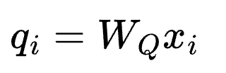
A key vector: 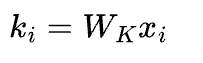
and a worth vector: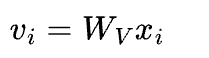
The eye rating between tokens i and j is: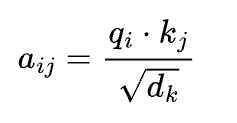
This rating determines how a lot token i “pays consideration to” token j.
In a bi-encoder, the question and doc are separate sequences. The question has tokens [q1,q2,…,qm] and the doc has [d1,d2,…,dn]. The eye matrix for the question is m×m and for the doc, n×n.
Particularly, there are zero phrases for: 
No question token ever attends to any doc token. The mannequin independently compresses every right into a single vector, then compares:
In a cross-encoder, the enter is one concatenated sequence [q1,…,qm,d1,…,dn] and The eye matrix is (m+n)×(m+n).
Now consideration phrases exists. In a really approximate method, the question token for “low cost” would attend to the doc token for “$500”, and the mannequin learns by means of coaching that this mixture means “not related.” This cross-attention occurs at each layer, constructing more and more summary relationships.
Multi-head consideration makes this much more highly effective. Every consideration head has its personal weight matrices, so totally different heads be taught to detect various kinds of relationships concurrently:
- One head may be taught lexical matching identical or comparable phrases
- One other may be taught semantic equivalence — “low cost” ↔ “funds”
- One other may be taught contradiction detection — “with out sugar” vs “comprises sugar”
- One other may be taught entity matching — the identical particular person or place referenced otherwise
On the finish of it, the outputs of all heads are concatenated and projected:
With a number of heads throughout a number of gamers, the mannequin has many unbiased heads inspecting query-document interplay at each stage of abstraction. Theoretically, that’s why cross-encoders are a lot extra expressive than bi-encoders.
However in fact the tradeoff is then compute: consideration prices extra and nothing is precomputed.
Sufficient concept. Let’s take a look at precise code.
I’ve constructed a companion repo with eight instance .py recordsdata that progress from primary implementation to distillation pipelines and full latency-profiled ColBERT implementations.
Each runs end-to-end and you’ll observe alongside as you learn by means of this part.
The primary is fairly easy:
def predict_scores(self, question: str, paperwork: checklist[str]) -> checklist[float]:
    pairs = [(query, doc) for doc in documents]
    scores = self._model.predict(pairs)
    return [float(s) for s in scores]
Below the hood, all my code does is pair the question with each doc and rating every pair by means of the cross-encoder:
def predict_scores(self, question: str, paperwork: checklist[str]) -> checklist[float]:
    pairs = [(query, doc) for doc in documents]
    scores = self._model.predict(pairs)
    return [float(s) for s in scores]
We start by feeding the question “How does photosynthesis work in vegetation?”, together with 10 paperwork.
- 5 are about photosynthesis
- 5 are noise about inventory markets, electrical autos, and historic Rome.
Naturally the photosynthesis paperwork float to the highest:
--- Reranked Order (10 outcomes) ---
  #1 (rating: 8.0888) [was #0] Photosynthesis is the method by which inexperienced vegetation convert...
  #2 (rating: 3.7970) [was #4] Throughout photosynthesis, carbon dioxide and water are transformed...
  #3 (rating: 2.4054) [was #6] Chloroplasts are the organelles the place photosynthesis takes...
  #4 (rating: 1.8762) [was #2] Vegetation use chlorophyll of their leaves to soak up mild...
  #5 (rating: -9.7185) [was #8] The sunshine-dependent reactions happen within the thylakoid...
  ...
  #10 (rating: -11.2886) [was #7] Machine studying algorithms can course of huge quantities...
And there’s actually nothing extra to it. The mannequin concatenates the question and doc as [CLS] question [SEP] doc [SEP], runs a ahead cross, and produces a relevance rating, order by descending.
Choosing the Proper Mannequin
The pure follow-up query: which cross-encoder ought to I take advantage of?
We benchmark 4 MS MARCO fashions on the identical question — from tiny to massive.
I run all 4 fashions run in parallel through ThreadPoolExecutor, so that you get leads to the time of the slowest mannequin reasonably than the sum. Right here’s what the output seems to be like:
--- Pace Comparability ---
Mannequin                                    Time (s)   Docs/sec
---------------------------------------- --------- ----------
ms-marco-MiniLM-L-12-v2                     0.560       14.3
ms-marco-electra-base                       0.570       14.0
ms-marco-MiniLM-L6-v2                       0.811        9.9
ms-marco-TinyBERT-L-2-v2                    1.036        7.7

--- Rating Order (by doc index) ---
  ms-marco-MiniLM-L6-v2:    0 → 2 → 4 → 6 → 7 → 1 → 3 → 5
  ms-marco-TinyBERT-L-2-v2: 2 → 4 → 0 → 6 → 5 → 3 → 1 → 7
  ms-marco-MiniLM-L-12-v2:  2 → 0 → 4 → 6 → 1 → 7 → 3 → 5
  ms-marco-electra-base:    2 → 4 → 0 → 6 → 1 → 3 → 7 → 5
All 4 fashions agree on the top-4 paperwork (0, 2, 4, 6), simply shuffled barely.
- TinyBERT is the odd one out , which places doc 5 (irrelevant) in fifth place whereas the others push it to the underside.
Usually talking:
- TinyBERT-L2-v2: extraordinarily quick however least correct — use for low-latency or edge eventualities.
- MiniLM-L6-v2: greatest steadiness of velocity and high quality — use because the default for many reranking duties.
- MiniLM-L12-v2: barely extra correct however slower — use when maximizing rating high quality issues.
- electra-base: (older) and bigger and slower with no clear benefit — usually not advisable over MiniLM.
High quality-Tuning: Making the Mannequin Perceive Your Area
Many pre-trained cross-encoders are nonetheless generalists, as a result of they’re educated on datasets like MS MARCO, which itself is an enormous dataset of Bing search queries paired with internet passages.
In case your area is one thing like authorized contracts, medical data, or cybersecurity incident reviews, the generalist mannequin may not rank your content material accurately. For instance, it doesn’t know that “pressure majeure” is a contract time period, not a army phrase.
High quality-tuning may simply do the trick.
There are two approaches relying on what sort of coaching information you’ve got, and the repo contains an instance of every.
When you’ve got comfortable scores, you should use MSE loss.
- A bigger trainer mannequin scores your query-document pairs, and the coed learns to breed these steady scores:
coach = MSEDistillationTrainer(student_model_name=STUDENT_MODEL, config=config)
output_path = coach.prepare(train_dataset)
When you’ve got binary labels, you should use BCE loss.
- Every coaching pair is solely marked related or not related:
finetuner = BCEFineTuner(model_name=BASE_MODEL, config=config)
output_path = finetuner.prepare(train_dataset)
Each approaches are fairly easy to arrange. Below the hood it’s so simple as:
        class BCEFineTuner:
    """High quality-tune a cross-encoder with binary cross-entropy loss.

    Appropriate for binary relevance judgments (related/not-relevant).

    Args:
        model_name: HuggingFace mannequin title to fine-tune.
        config: Coaching configuration.

    Instance:
        >>> finetuner = BCEFineTuner("cross-encoder/ms-marco-MiniLM-L6-v2")
        >>> finetuner.prepare(train_dataset)
    """

    def __init__(
        self,
        model_name: str = "cross-encoder/ms-marco-MiniLM-L6-v2",
        config: TrainingConfig | None = None,
    ) -> None:
        self._config = config or TrainingConfig()
        self._model = CrossEncoder(model_name, num_labels=1)
        self._model_name = model_name

    @property
    def mannequin(self) -> CrossEncoder:
        """Return the mannequin being fine-tuned."""
        return self._model

    def prepare(
        self,
        train_dataset: Dataset,
        eval_dataset: Dataset | None = None,
    ) -> Path:
        """Run BCE fine-tuning.

        The dataset ought to have columns: "sentence1", "sentence2", "label"
        the place "label" is 0 or 1.

        Args:
            train_dataset: Dataset with query-document-label triples.
            eval_dataset: Non-obligatory analysis dataset.

        Returns:
            Path to the saved mannequin listing.
        """
        from sentence_transformers.cross_encoder.losses import BinaryCrossEntropyLoss

        loss = BinaryCrossEntropyLoss(self._model)
        args = self._config.to_training_arguments(has_eval=eval_dataset isn't None)

        coach = CrossEncoderTrainer(
            mannequin=self._model,
            args=args,
            train_dataset=train_dataset,
            eval_dataset=eval_dataset,
            loss=loss,
        )
        coach.prepare()

        output_path = Path(self._config.output_dir) / "final_model"
        self._model.save(str(output_path))
        return output_path
The fascinating half is the analysis, and particularly what occurs while you throw adversarial distractors on the mannequin.
After coaching, I take a look at on circumstances the place every question is paired with a related doc and a tough distractor. In my definition, a tough distractor is a doc that shares key phrases however is definitely about one thing totally different. For this analysis, a “cross” simply means the mannequin scored the related doc increased:
b_scores = base_model.predict_scores(case.question, docs)
f_scores = fine_tuned.predict_scores(case.question, docs)

b_pass = b_scores[0] > b_scores[1]
f_pass = f_scores[0] > f_scores[1]
We break up the eval into ‘SEEN’ subjects (identical subjects as coaching, totally different examples) and ‘UNSEEN’ subjects (fully new). The ‘UNSEEN’ break up is the one which issues as a result of it proves the mannequin discovered the area reasonably than memorising the coaching set. Simply as we might for many ML analysis workflows.
Right here’s the MSE fine-tuning end result:
Base Mannequin          High quality-Tuned
  Total accuracy:          15/20 ( 75%)       20/20 (100%)
  Seen subjects:                7/10              10/10
  Unseen subjects:              8/10              10/10

High quality-tuning mounted 5 case(s) the bottom mannequin obtained flawed.
  Common confidence: 316x enchancment (hole: +0.0001 -> +0.0386)
From the above, we see that fine-tuning mounted the 5 circumstances the place the bottom mannequin obtained flawed, and there was a big enchancment in common confidence. The bottom mannequin’s right solutions had been barely right (hole of +0.0001), however after fine-tuning, the hole widens to +0.0386. So, the mannequin isn’t simply getting the proper reply extra typically, it’s getting it with fairly a little bit of conviction.
The BCE fine-tuning end result on authorized information (Instance 4) is even clearer:
Base Mannequin      High quality-Tuned
  Total accuracy:           6/20 ( 30%)       19/20 ( 95%)
  Seen subjects:                2/10               9/10
  Unseen subjects:              4/10              10/10
Accuracy rising from 30% to 95% signifies that the unique base mannequin was one way or the other worse than random on authorized paperwork. After fine-tuning on simply 72 coaching pairs , 12 authorized subjects with 6 pairs every, the mannequin will get 19 out of 20 proper. And spot that unseen subjects went from 4/10 to 10/10. In a way it learnt the area of authorized reasoning, not simply the coaching examples.
The output in my repo marks every case the place <-- fine-tuning mounted this,primarily the place the bottom mannequin failed however the fine-tuned mannequin obtained it proper.
Right here’s one illustrative instance:
[SEEN  ] What qualifies as wrongful termination?
           Related:   Terminating an worker in retaliation for reporting security viola...
           Distractor: The wrongful termination of the TV collection certified it for a fan ...
           Base:  FAIL  (hole: -8.3937)   High quality-tuned:  PASS  (hole: +3.8407)
           <-- fine-tuning mounted this
The bottom mannequin confidently selected the TV collection distractor attributable to key phrase matches. After fine-tuning, it accurately identifies the employment legislation doc as a substitute.
One factor I actually need to name out, as I used to be figuring all of this out, is that your distractors can strongly affect what your mannequin learns. Instance 4 trains on authorized information the place the distractors come from associated authorized subjects, for instance, a contract dispute distractor for a tort case, a regulatory compliance distractor for a legal legislation question. (No I’m not a authorized knowledgeable I obtained AI to generate these examples for me)
The problem is that these examples share vocabulary like “plaintiff”, “jurisdiction”, “statute”. Should you used cooking recipes as distractors for authorized queries, the mannequin would be taught nothing as a result of it might already inform these aside. So the exhausting negatives from the identical area are what pressure it to be taught fine-grained distinctions.
In some ways, these shares similarities with how I’ve all the time seen imbalanced datasets when doing supervised coaching. The best way you choose (downsample) your majority class is extraordinarily necessary. Choose the observations that look actually just like the minority class, and you’ve got your self a dataset that may prepare a extremely highly effective (exact) discriminator.
Semantic Question Caching
In manufacturing, customers ask the identical query a dozen other ways. “How do I reset my password?” and “I forgot my password, how do I alter it?” ought to ideally return identical cached outcomes reasonably than triggering two separate and costly search, reranking and era operations.
The concept is straightforward: use a cross-encoder fine-tuned on one thing just like the Quora duplicate query dataset to detect semantic duplicates at question time.
def find_duplicate(self, question: str) -> tuple[CacheEntry | None, float]:
    if not self._cache:
        return None, 0.0

...

cached_queries = [entry.query for entry in self._cache]
    scores = self._reranker.predict_scores(question, cached_queries)
    best_idx = max(vary(len(scores)), key=lambda i: scores[i])
    best_score = scores[best_idx]
    if best_score >= self._threshold:
        return self._cache[best_idx], best_score
    return None, best_score
Each incoming question will get scored towards every part already within the cache. If the most effective rating exceeds a threshold, it’s a reproduction, so return the cached rating. If not, run the total reranking pipeline and cache the brand new end result.
To check this correctly, we simulate 50 consumer queries throughout 12 subjects. Every matter begins with a “seed” question that misses the cache, adopted by paraphrase variants that ought to hit:
("How do I reset my password?", None),            # MISS - first time
("How can I reset my password?", 1),               # HIT → question #1
("How one can reset my password?", 1),                  # HIT → question #1
("I forgot my password, how do I alter it?", 1),  # HIT → question #1
The output exhibits the cache increase over time. Early queries are all misses, however as soon as the cache has 12 seed queries, every part that follows is a success:
#  Outcome    Time  Question                                            Matched
    1  ✗ MISS      0ms  How do I reset my password?                      -
    2  ✗ MISS   2395ms  How do I export my information from the platform?       -
    ...
    4  ✓ HIT     844ms  How can I reset my password?                     → #01 (0.99)
    ...
   25  ✓ HIT      61ms  I forgot my password, how do I alter it?        → #01 (0.99)
   ...
   49  ✓ HIT      17ms  I must reset my password, how?                → #01 (0.92)
   50  ✓ HIT      25ms  Can I add or take away individuals from my workforce?         → #12 (0.93)
The bottom-truth labels allow us to compute precision and recall:
Whole queries:        50
  Cache hits:           38   (anticipated 38)
  Cache misses:         12   (anticipated 12)

HIT  precision:       38 / 38  (100%)
  MISS precision:       12 / 12  (100%)
  Total accuracy:     50 / 50  (100%)
  With out caching: 50 rankings wanted.  With caching: 12 carried out.  76% financial savings.
100% accuracy, and each single hit is right, each single miss is genuinely new. Consequently, we keep away from 76% (38/50) of rating operations in our take a look at dataset.
In fact, the cache comparability itself has O(n) price towards the cache dimension. In an actual system you’d most likely need to restrict the cache dimension or use a extra environment friendly index. However the core thought of utilizing a cross-encoder educated for paraphrase detection to gate costly downstream operations is sound and production-tested.
The Multi-Stage Funnel
Bringing all of it collectively in manufacturing, you’ll be able to construct a funnel the place every stage trades velocity for precision, and the candidate set shrinks at each step.
For instance, 50 paperwork → 20 (bi-encoder) → 10 (cross-encoder) → 5 (LLM)
The implementation is fairly easy:
def run_pipeline(self, question, paperwork, stage1_k=20, stage2_k=10, stage3_k=5):
    s1 = self.stage1_biencoder(question, paperwork, top_k=stage1_k)
    s2 = self.stage2_crossencoder(question, paperwork, s1.doc_indices, top_k=stage2_k)
    s3 = self.stage3_llm(question, paperwork, s2.doc_indices, top_k=stage3_k)
    return [s1, s2, s3]
Stage 1 is a bi-encoder: encode question and paperwork independently, rank by cosine similarity. Low cost sufficient for 1000’s of paperwork. Take the highest 20.
Stage 2 is the cross-encoder we’ve been discussing. Rating the query-document pairs with full cross-attention. Take the highest 10.
Stage 3 is an non-compulsory step the place we are able to utilise an LLM to do list-wise reranking. In contrast to the cross-encoder which scores every pair independently, the LLM sees all 10 candidates directly in a single immediate and produces a world ordering. That is the one stage that may cause about relative relevance: “Doc A is best than Doc B as a result of…”
In my code, the LLM stage calls OpenRouter and makes use of structured output to ensure parseable JSON again:
RANKING_SCHEMA = {
    "title": "ranking_response",
    "strict": True,
    "schema": {
        "sort": "object",
        "properties": {
            "rating": {
                "sort": "array",
                "objects": {"sort": "integer"},
            },
        },
        "required": ["ranking"],
        "additionalProperties": False,
    },
}
The take a look at corpus has 50 paperwork with ground-truth relevance tiers: extremely related, partially related, distractors, and irrelevant.
The output exhibits noise getting filtered at every stage:
Stage                                          Related  Partial    Noise  Precision
  Bi-Encoder (all-MiniLM-L6-v2)                     10/20     7/20     3/20        85%
  Cross-Encoder (cross-encoder/ms-marco-MiniLM...)   10/10     0/10     0/10       100%
  LLM (google/gemini-2.0-flash-001)                   5/5      0/5      0/5        100%

Whole pipeline time: 2243ms
The bi-encoder’s top-20 let by means of 3 noise paperwork and seven partial matches. The cross-encoder eradicated all of them, 10 for 10 on related paperwork. The LLM preserved that precision whereas reducing to the ultimate 5.
The timing breakdown is value noting too: the bi-encoder took 176ms to attain all 50 paperwork, the cross-encoder took 33ms for 20 pairs, the LLM took 2034ms for a single API name, by far the slowest stage, however it solely ever sees 10 paperwork.
Information Distillation: Instructing the Bi-Encoder to Suppose Like a Cross-Encoder
The multi-stage funnel works, however the generic bi-encoder was by no means educated in your area information. It retrieves primarily based on surface-level semantic similarity, which suggests it would nonetheless miss related paperwork or let by means of irrelevant ones.
What when you may educate the bi-encoder to rank just like the cross-encoder?
That’s the essence of distillation. The cross-encoder (trainer) scores your coaching pairs. The bi-encoder (scholar) learns to breed these scores. At inference time, you throw away the trainer and simply use the quick scholar.
distiller = CrossEncoderDistillation(
    teacher_model_name="cross-encoder/ms-marco-MiniLM-L6-v2",
    student_model_name="all-MiniLM-L6-v2",
)

output_path = distiller.prepare(
    training_pairs=TRAINING_PAIRS,
    epochs=4,
    batch_size=16,
)
The prepare technique that I’ve applied mainly seems to be like this:
train_dataset = Dataset.from_dict({
    "sentence1": [q for q, _, _ in training_pairs],
    "sentence2": [d for _, d, _ in training_pairs],
    "rating": [s for _, _, s in training_pairs],
})

loss = losses.CosineSimilarityLoss(self._student)

args = SentenceTransformerTrainingArguments(
    output_dir=output_dir,
    num_train_epochs=epochs,
    per_device_train_batch_size=batch_size,
    learning_rate=2e-5,
    warmup_steps=0.1,
    logging_steps=5,
    logging_strategy="steps",
    save_strategy="no",
)

coach = SentenceTransformerTrainer(
    mannequin=self._student,
    args=args,
    train_dataset=train_dataset,
    loss=loss,
)
coach.prepare()
To show that this truly works, we selected a intentionally tough area: cybersecurity. In cybersecurity, each doc shares the identical vocabulary. Assault, vulnerability, exploit, malicious, payload, compromise, breach, these phrases seem in paperwork about SQL injection, phishing, buffer overflows, and ransomware alike. A generic bi-encoder maps all of them to roughly the identical area of embedding area and so it can’t inform them aside.
The AI-generated coaching dataset I’ve makes use of exhausting distractors from confusable subtopics:
- SQL injection ↔ command injection (each “injection assaults”)
- XSS ↔ CSRF (each client-side internet assaults)
- phishing ↔ pretexting (each social engineering)
- buffer overflow ↔ use-after-free (each reminiscence corruption)
After coaching, we run a three-way comparability on 30 take a look at circumstances, 15 from assault varieties the mannequin educated on, and 15 from assault varieties it’s by no means seen:
t_scores = trainer.generate_teacher_scores(case.question, docs)   # cross-encoder
b_scores = trainer.generate_student_scores(case.question, docs)   # base bi-encoder
d_scores = educated.generate_student_scores(case.question, docs)   # distilled bi-encoder
Right here’s what the output seems to be like for a typical case:
[SEEN  ] What's a DDoS amplification assault?
           Trainer:    rel=+5.5097  dist=-6.5875
           Base:       PASS  (rel=0.7630  dist=0.3295  hole=+0.4334)
           Distilled:  PASS  (rel=0.8640  dist=0.2481  hole=+0.6160)
The trainer (cross-encoder) gives the bottom fact scores. Each the bottom and distilled bi-encoders get this one proper, however take a look at the hole: the distilled mannequin is 42% extra assured. In a means, it pushes the related doc farther from the distractor in embedding area.
The abstract of all assessments tells the total story of efficiency:
Base Pupil     Distilled Pupil
  Total accuracy:          29/30 ( 96.7%)       29/30 ( 96.7%)
  Seen subjects:               15/15                 15/15
  Unseen subjects:             14/15                 14/15
  Avg relevance hole:              +0.2679               +0.4126
Similar accuracy, however 1.5x wider confidence margins. Each fashions fail on one edge case : the “memory-safe languages” question, the place even the cross-encoder trainer disagreed with the anticipated label. However throughout the board, the distilled scholar separates related from irrelevant paperwork extra decisively.
This is without doubt one of the extra modern and doubtlessly impactful approach that I’ve been experimenting on this venture: you get cross-encoder high quality at bi-encoder velocity, a minimum of on your particular area… assuming you’ve got sufficient information. So assume exhausting about what sorts of information you’ll need to accumulate, label, and course of when you assume this type of distillation can be helpful to you down the street.
ColBERT-like Late Interplay
So now now we have a spectrum. On one finish, bi-encoders are quick, can precompute, however there isn’t a interplay between question and doc tokens. On the opposite finish, cross-encoders have full interplay, are extra correct, however nothing is precomputable. Is there one thing in between?
ColBERT (COntextualized Late interplay over BERT) is one such center floor. The title tells you the structure. “Contextualised” means the token embeddings are context-dependent (in contrast to word2vec the place “financial institution” all the time maps to the identical vector, BERT’s illustration of “financial institution” adjustments relying on whether or not it seems close to “river” or “account”). “Late interplay” means question and doc are encoded individually and solely work together on the very finish, through operationally cheap dot merchandise reasonably than costly transformer consideration. And “BERT” is the spine encoder.
That “late” half is the important thing distinction. A cross-encoder does early interplay within the sense that question and doc tokens attend to one another contained in the transformer. A bi-encoder does no interplay, simply cosine similarity between two pooled vectors. ColBERT sits in between.
When a bi-encoder encodes a sentence, it produces one embedding per token, then swimming pools them, sometimes by averaging right into a single vector, for instance:
"How do quantum computer systems obtain speedup?"
→ 9 token embeddings (every 384-dim)
→ imply pool
→ 1 vector (384-dim): [0.12, -0.34, 0.56, …]
That single vector is what will get in contrast through cosine similarity. It’s quick and it really works, however the pooling step crushes the richness of knowledge. The phrase “quantum” had its personal embedding, and so did “speedup.” After imply pooling, their particular person alerts are averaged along with filler tokens like “do” and “how.” The ensuing vector is a blurry abstract of the entire sentence.
The ColBERT-like late interplay skips the pooling by retaining all 9 token embeddings:
"How do quantum computer systems obtain speedup?"
→
"how" → [0.05, -0.21, …] (384-dim)
"quantum" → [0.89, 0.42, …] (384-dim)
"computer systems" → [0.67, 0.31, …] (384-dim)
"speedup" → [0.44, 0.78, …] (384-dim)

… 9 tokens complete → (9 × 384) matrix
Similar for the paperwork we’re evaluating towards. A 30-token doc turns into a (30 × 384) matrix as a substitute of a single vector.
Now you want a technique to rating the match between a (9 × 384) question matrix and a (30 × 384) doc matrix. That’s MaxSim.
For every question token, discover its best-matching doc token (the one with the very best cosine similarity) and take that most. Then sum all of the maxima throughout question tokens.
@staticmethod
def _maxsim(q_embs, d_embs):
    sim_matrix = torch.matmul(q_embs, d_embs.T)
    max_sims = sim_matrix.max(dim=1).values
return float(max_sims.sum())
Let’s hint by means of the mathematics. The matrix multiply `(9 × 384) × (384 × 30)` produces a `9 × 30` similarity matrix. Every cell tells you ways comparable one question token is to at least one doc token. Then `.max(dim=1)` takes the most effective doc match for every question token , 9 values. Then `.sum()` provides them up into one rating.
The question token “quantum” scans all 30 doc tokens and finds its greatest match , most likely one thing like “qubits” with similarity ~0.85. The question token “speedup” finds one thing like “quicker” at ~0.7. In the meantime, filler tokens like “how” and “do” match weakly towards every part (~0.1). Sum these 9 maxima and also you get a rating like 9.93, simply for example.
Why does this work higher than a single pooled vector? As a result of the token-level matching preserves fine-grained sign. The question token “quantum” can particularly latch onto the doc token “qubit” through their embedding similarity, despite the fact that they’re totally different phrases.
With imply pooling, that exact match will get averaged away right into a blurry centroid the place “quantum” and “how” contribute equally.
The important thing benefit, and the rationale you’d take into account ColBERT-like late interplay in manufacturing, is pre-indexing. As a result of paperwork are encoded independently of the question, you’ll be able to encode your whole corpus offline and cache the token embeddings:
def index(self, paperwork):
  self._doc_embeddings = []
  for doc in paperwork:
    emb = self._model.encode(doc, output_value="token_embeddings")
    tensor = torch.nn.useful.normalize(torch.tensor(emb), dim=-1)
    self._doc_embeddings.append(tensor)
At search time, you solely encode the question, one ahead cross, after which run dot merchandise towards the cached embeddings. The cross-encoder would wish to encode all 60 (question, doc) pairs from scratch.
How shut does it get to cross-encoder high quality? Right here’s the abstract from operating 10 queries throughout a 60-document corpus spanning quantum computing, vaccines, ocean chemistry, renewable vitality, ML, astrophysics, genetics, blockchain, microbiology, and geography:
Rating settlement (ColBERT vs cross-encoder floor fact):
Avg Kendall's tau: +0.376
Avg top-3 overlap: 77%
Avg top-5 overlap: 92%

Latency breakdown:
ColBERT indexing: 358.7ms (one-time, 60 docs)
ColBERT queries: 226.4ms complete (22.6ms avg per question)
Cross-encoder: 499.1ms complete (49.9ms avg per question)
Question speedup: 2.2x quicker
92% top-5 overlap, so many of the occasions it’s retrieving the identical paperwork; it simply often shuffles the within-topic ordering. For many functions, that’s ok, and at 2.2x quicker per question.
And the actual energy comes while you observe what occurs beneath load.
I collected 100 actual processing time samples for every system, then simulated a single-server queue at rising QPS ranges. Requests arrive at mounted intervals, queue up if the server is busy, and we measure the whole response time (queue wait + processing):
===========================================================================
LATENCY PROFILING
===========================================================================

  Uncooked processing time (100 samples per system):
                       p50     p95     p99    p99.9     max
    ───────────────────────────────────────────────────────
    ColBERT           20.4ms    30.8ms    54.2ms     64.3ms    64.3ms
    Cross-encoder     45.2ms    56.7ms    69.0ms     72.1ms    72.1ms

===========================================================================
QPS SIMULATION (single-server queue, 1000 requests per stage)
===========================================================================

  Response time = queue wait + processing time.
  When QPS exceeds throughput, requests queue and tail latencies explode.

  QPS: 5 (ColBERT util: 10%, cross-encoder util: 23%)
                       p50     p95     p99    p99.9     max
    ───────────────────────────────────────────────────────
    ColBERT           20.4ms    30.8ms    54.2ms     64.3ms    64.3ms
    Cross-encoder     45.2ms    56.7ms    69.0ms     72.1ms    72.1ms

  QPS: 10 (ColBERT util: 20%, cross-encoder util: 45%)
                       p50     p95     p99    p99.9     max
    ───────────────────────────────────────────────────────
    ColBERT           20.4ms    30.8ms    54.2ms     64.3ms    64.3ms
    Cross-encoder     45.2ms    56.7ms    69.0ms     72.1ms    72.1ms

  QPS: 20 (ColBERT util: 41%, cross-encoder util: 90%)
                       p50     p95     p99    p99.9     max
    ───────────────────────────────────────────────────────
    ColBERT           20.4ms    34.0ms    62.9ms     64.3ms    64.3ms
    Cross-encoder     50.8ms    74.8ms    80.9ms     82.8ms    82.8ms

  QPS: 30 (ColBERT util: 61%, cross-encoder util: 136%)
                       p50     p95     p99    p99.9     max
    ───────────────────────────────────────────────────────
    ColBERT           20.7ms    49.1ms    67.3ms     79.6ms    79.6ms
    Cross-encoder   6773.0ms 12953.5ms 13408.0ms  13512.6ms 13512.6ms

  QPS: 40 (ColBERT util: 82%, cross-encoder util: 181%)
                       p50     p95     p99    p99.9     max
    ───────────────────────────────────────────────────────
    ColBERT           23.0ms    67.8ms    84.0ms     87.9ms    87.9ms
    Cross-encoder  10931.3ms 20861.8ms 21649.7ms  21837.6ms 21837.6ms
Should you take a look at 30 QPS, you see that the cross-encoder’s utilization exceeds 100%, requests arrive each 33ms however every takes 45ms to course of. Each request provides about 12ms of queue debt. After 500 requests, the queue has accrued over 6 seconds of wait time. That’s your p50, so half your customers are ready practically 7 seconds.
In the meantime, ColBERT-like late interplay at 61% utilisation is barely sweating at 20.7ms p50, and each percentile roughly the place it was at idle.
At 40 QPS, the cross-encoder’s p99.9 is over 21 seconds. ColBERT’s p50 is 23ms.
So that is one thing to consider as nicely in manufacturing, you may need to select your reranking structure primarily based in your QPS funds, not simply your accuracy necessities.
A caveat: this can be a ColBERT-like implementation. It demonstrates the MaxSim mechanism utilizing `all-MiniLM-L6-v2`, which is a general-purpose sentence transformer. Actual ColBERT deployments use fashions particularly educated for token-level late interplay retrieval, like `colbert-ir/colbertv2.0`.
The place Does This Depart Us?
These examples illustrate choices on retrieval and reranking:
- Cross-encoder (uncooked): Sluggish, highest high quality. Use for small candidate units beneath 100 docs.
- High quality-tuned cross-encoder: Sluggish, highest high quality on your area. Use when basic fashions carry out poorly on area content material.
- Semantic caching: Prompt on cache hit, identical high quality as underlying ranker. Use for high-traffic methods with repeated queries.
- Multi-stage funnel: Sluggish per question, scales to massive corpora, efficiency close to cross-encoder
- Distilled bi-encoder: Quick, close to cross-encoder high quality. Use as first stage of a funnel or for domain-specific retrieval.
- ColBERT-like (late interplay): Medium velocity, close to cross-encoder high quality. Use for high-QPS providers the place tail latency issues.
A mature search system may mix any of them: a distilled bi-encoder for first-pass retrieval, a cross-encoder for reranking the highest candidates, semantic caching to skip redundant work, and ColBERT-like interplay as a fallback when the latency funds is tight.
All of the code is obtainable at https://github.com/ianhohoho/cross-encoder-and-reranking-demo. The truth is, each instance runs end-to-end with out API keys required besides Instance 6, which calls an LLM by means of OpenRouter for the list-wise reranking stage.
Should you’ve made it to the tip, I’d love to listen to the way you’re dealing with retrieval and reranking in manufacturing, what’s your stack appear to be? Are you operating a multi-stage funnel, or is a single bi-encoder doing the job?
I’m all the time glad to listen to your ideas on the approaches I’ve laid out above, and be happy to make solutions to my implementation as nicely!
Let’s join! 🤝🏻 with me on LinkedIn or take a look at my site



