


For my charts I take advantage of the Olympic Historical past dataset from Olympedia.org shared by Joseph Chen. Kaguru Public area license included.

It comprises the outcomes of Olympic competitions at aggressive to athlete stage from Athens 1896 to Beijing 2022. After EDA (Exploratory Knowledge Evaluation), I’ve transformed this right into a dataset detailing the variety of feminine athletes per yr in every sport/sport. The concept of my bubble chart is to indicate which sports activities have athletes with a 50/50 ratio of feminine to male and the way that has modified over time.
My plot information consists of two totally different datasets, one for annually. 2020 and 1996For every information set, we calculated the sum of athletes who participated in every occasion. (Athletes_Total) And what number of the overall variety of athletes (male + feminine) does that characterize? (distinction)See the screenshot of the info beneath.

This is my strategy to visualizing this:
- Dimension ratio. Use the bubble radius to check the variety of athletes per sport, with bigger bubbles representing extremely aggressive occasions equivalent to observe and area.
- Multivariate interpretationShade is used to characterize feminine illustration: a light-weight inexperienced bubble represents an occasion with a 50/50 cut up, equivalent to hockey.
That is my place to begin (utilizing the code and strategy above).

A fast repair is to extend the scale of the image and if the scale shouldn’t be over 250 change the label to empty so the phrases do not seem exterior the bubble.
fig, ax = plt.subplots(figsize=(12,8),subplot_kw=dict(side="equal"))#Labels edited straight in dataset

Effectively, at the very least I can learn it now. However why? Athletics pink and boxing Blue? Let’s add a legend that explains the connection between colours and feminine illustration.
This isn’t a traditional bar graph, plt.legend() It will not assist right here.
Utilizing matplotlib Annotation Bbox, you may create a rectangle (or circle) to indicate what every shade means. It’s also possible to do the identical to indicate a bubble scale.
import matplotlib.pyplot as plt
from matplotlib.offsetbox import (AnnotationBbox, DrawingArea,
TextArea,HPacker)
from matplotlib.patches import Circle,Rectangle# That is an instance for one part of the legend
# Outline the place the annotation (legend) might be
xy = [50, 128]
# Create your coloured rectangle or circle
da = DrawingArea(20, 20, 0, 0)
p = Rectangle((10 ,10),10,10,shade="#fc8d62ff")
da.add_artist(p)
# Add textual content
textual content = TextArea("20%", textprops=dict(shade="#fc8d62ff", dimension=14,fontweight='daring'))
# Mix rectangle and textual content
vbox = HPacker(kids=[da, text], align="high", pad=0, sep=3)
# Annotate each in a field (change alpha if you wish to see the field)
ab = AnnotationBbox(vbox, xy,
xybox=(1.005, xy[1]),
xycoords='information',
boxcoords=("axes fraction", "information"),
box_alignment=(0.2, 0.5),
bboxprops=dict(alpha=0)
)
#Add to your bubble chart
ax.add_artist(ab)
I additionally added a subtitle and textual content description beneath the graph. plt.Textual content()

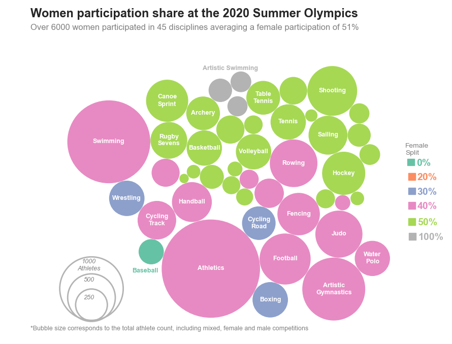
Clear and user-friendly interpretation of the graphs:
- Many of the bubbles are mild inexperienced → inexperienced means 50% feminine → Most Olympic sports activities have a good 50/50 cut up between feminine and male athletes (Yay🙌)
- The one sport highlighted in darkish inexperienced (baseball) doesn’t embody ladies.
- Three sports activities are completely female-represented, however the variety of athletes is pretty small.
- The sports activities with essentially the most athletes (swimming, observe and area, and gymnastics) have an almost 50/50 cut up.
