On this tutorial, I wish to present you the best way to downsample a stream of sensor knowledge utilizing solely Python (and Redpanda as a message dealer). The aim is to indicate you the way easy stream processing will be, and that you just don’t want a heavy-duty stream processing framework to get began.
Till lately, stream processing was a fancy job that often required some Java experience. However regularly, the Python stream processing ecosystem has matured and there are just a few extra choices accessible to Python builders — reminiscent of Faust, Bytewax and Quix. Later, I’ll present a bit extra background on why these libraries have emerged to compete with the present Java-centric choices.
However first let’s get to the duty at hand. We are going to use a Python libary referred to as Quix Streams as our stream processor. Quix Streams is similar to Faust, however it has been optimized to be extra concise in its syntax and makes use of a Pandas like API referred to as StreamingDataframes.
You possibly can set up the Quix Streams library with the next command:
pip set up quixstreams
What you’ll construct
You’ll construct a easy software that may calculate the rolling aggregations of temperature readings coming from numerous sensors. The temperature readings will are available at a comparatively excessive frequency and this software will combination the readings and output them at a decrease time decision (each 10 seconds). You possibly can consider this as a type of compression since we don’t wish to work on knowledge at an unnecessarily excessive decision.
You possibly can entry the whole code in this GitHub repository.
This software contains code that generates artificial sensor knowledge, however in a real-world situation this knowledge might come from many sorts of sensors, reminiscent of sensors put in in a fleet of automobiles or a warehouse stuffed with machines.
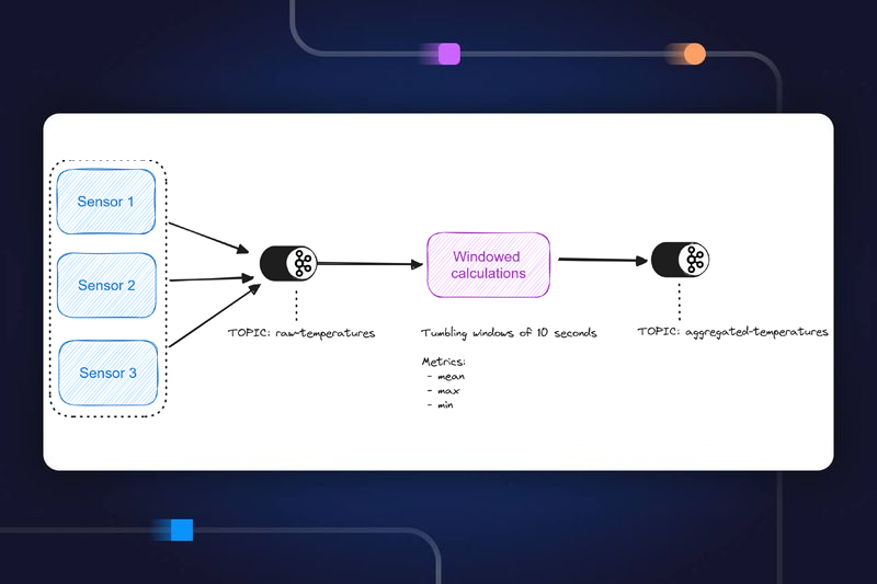
Right here’s an illustration of the essential structure:

The earlier diagram displays the primary parts of a stream processing pipeline: You could have the sensors that are the knowledge producers, Redpanda because the streaming knowledge platform, and Quix because the stream processor.
Knowledge producers
These are bits of code which can be connected to methods that generate knowledge reminiscent of firmware on ECUs (Engine Management Models), monitoring modules for cloud platforms, or internet servers that log person exercise. They take that uncooked knowledge and ship it to the streaming knowledge platform in a format that that platform can perceive.
Streaming knowledge platform
That is the place you set your streaming knowledge. It performs kind of the identical function as a database does for static knowledge. However as a substitute of tables, you employ subjects. In any other case, it has related options to a static database. You’ll wish to handle who can eat and produce knowledge, what schemas the info ought to adhere to. In contrast to a database although, the info is consistently in flux, so it’s not designed to be queried. You’d often use a stream processor to remodel the info and put it elsewhere for knowledge scientists to discover or sink the uncooked knowledge right into a queryable system optimized for streaming knowledge reminiscent of RisingWave or Apache Pinot. Nevertheless, for automated methods which can be triggered by patterns in streaming knowledge (reminiscent of suggestion engines), this isn’t a super resolution. On this case, you undoubtedly wish to use a devoted stream processor.
Stream processors
These are engines that carry out steady operations on the info because it arrives. They may very well be in comparison with simply common previous microservices that course of knowledge in any software again finish, however there’s one large distinction. For microservices, knowledge arrives in drips like droplets of rain, and every “drip” is processed discreetly. Even when it “rains” closely, it’s not too laborious for the service to maintain up with the “drops” with out overflowing (consider a filtration system that filters out impurities within the water).
For a stream processor, the info arrives as a steady, huge gush of water. A filtration system can be rapidly overwhelmed except you modify the design. I.e. break the stream up and route smaller streams to a battery of filtration methods. That’s type of how stream processors work. They’re designed to be horizontally scaled and work in parallel as a battery. And so they by no means cease, they course of the info constantly, outputting the filtered knowledge to the streaming knowledge platform, which acts as a type of reservoir for streaming knowledge. To make issues extra difficult, stream processors typically must preserve observe of information that was obtained beforehand, reminiscent of within the windowing instance you’ll check out right here.
Notice that there are additionally “knowledge customers” and “knowledge sinks” — methods that eat the processed knowledge (reminiscent of entrance finish purposes and cell apps) or retailer it for offline evaluation (knowledge warehouses like Snowflake or AWS Redshift). Since we received’t be overlaying these on this tutorial, I’ll skip over them for now.
On this tutorial, I’ll present you the best way to use a neighborhood set up of Redpanda for managing your streaming knowledge. I’ve chosen Redpanda as a result of it’s very simple to run regionally.
You’ll use Docker compose to rapidly spin up a cluster, together with the Redpanda console, so ensure you have Docker put in first.
First, you’ll create separate recordsdata to supply and course of your streaming knowledge. This makes it simpler to handle the operating processes independently. I.e. you possibly can cease the producer with out stopping the stream processor too. Right here’s an outline of the 2 recordsdata that you just’ll create:
- The stream producer:
sensor_stream_producer.pyGenerates artificial temperature knowledge and produces (i.e. writes) that knowledge to a “uncooked knowledge” supply matter in Redpanda. Similar to the Faust instance, it produces the info at a decision of roughly 20 readings each 5 seconds, or round 4 readings a second. - The stream processor:
sensor_stream_processor.pyConsumes (reads) the uncooked temperature knowledge from the “supply” matter, performs a tumbling window calculation to lower the decision of the info. It calculates the typical of the info obtained in 10-second home windows so that you get a studying for each 10 seconds. It then produces these aggregated readings to theagg-temperaturesmatter in Redpanda.
As you possibly can see the stream processor does many of the heavy lifting and is the core of this tutorial. The stream producer is a stand-in for a correct knowledge ingestion course of. For instance, in a manufacturing situation, you may use one thing like this MQTT connector to get knowledge out of your sensors and produce it to a subject.
- For a tutorial, it’s less complicated to simulate the info, so let’s get that arrange first.
You’ll begin by creating a brand new file referred to as sensor_stream_producer.py and outline the primary Quix software. (This instance has been developed on Python 3.10, however totally different variations of Python 3 ought to work as effectively, so long as you’ll be able to run pip set up quixstreams.)
Create the file sensor_stream_producer.py and add all of the required dependencies (together with Quix Streams)
from dataclasses import dataclass, asdict # used to outline the info schema
from datetime import datetime # used to handle timestamps
from time import sleep # used to decelerate the info generator
import uuid # used for message id creation
import json # used for serializing knowledgefrom quixstreams import Software
Then, outline a Quix software and vacation spot matter to ship the info.
app = Software(broker_address='localhost:19092')destination_topic = app.matter(identify='raw-temp-data', value_serializer="json")
The value_serializer parameter defines the format of the anticipated supply knowledge (to be serialized into bytes). On this case, you’ll be sending JSON.
Let’s use the dataclass module to outline a really primary schema for the temperature knowledge and add a operate to serialize it to JSON.
@dataclass
class Temperature:
ts: datetime
worth: intdef to_json(self):
# Convert the dataclass to a dictionary
knowledge = asdict(self)
# Format the datetime object as a string
knowledge['ts'] = self.ts.isoformat()
# Serialize the dictionary to a JSON string
return json.dumps(knowledge)
Subsequent, add the code that might be chargeable for sending the mock temperature sensor knowledge into our Redpanda supply matter.
i = 0
with app.get_producer() as producer:
whereas i < 10000:
sensor_id = random.selection(["Sensor1", "Sensor2", "Sensor3", "Sensor4", "Sensor5"])
temperature = Temperature(datetime.now(), random.randint(0, 100))
worth = temperature.to_json()print(f"Producing worth {worth}")
serialized = destination_topic.serialize(
key=sensor_id, worth=worth, headers={"uuid": str(uuid.uuid4())}
)
producer.produce(
matter=destination_topic.identify,
headers=serialized.headers,
key=serialized.key,
worth=serialized.worth,
)
i += 1
sleep(random.randint(0, 1000) / 1000)
This generates 1000 information separated by random time intervals between 0 and 1 second. It additionally randomly selects a sensor identify from an inventory of 5 choices.
Now, check out the producer by operating the next within the command line
python sensor_stream_producer.py
You must see knowledge being logged to the console like this:
[data produced]
When you’ve confirmed that it really works, cease the method for now (you’ll run it alongside the stream processing course of later).
The stream processor performs three principal duties: 1) eat the uncooked temperature readings from the supply matter, 2) constantly combination the info, and three) produce the aggregated outcomes to a sink matter.
Let’s add the code for every of those duties. In your IDE, create a brand new file referred to as sensor_stream_processor.py.
First, add the dependencies as earlier than:
import os
import random
import json
from datetime import datetime, timedelta
from dataclasses import dataclass
import logging
from quixstreams import Softwarelogging.basicConfig(degree=logging.INFO)
logger = logging.getLogger(__name__)
Let’s additionally set some variables that our stream processing software wants:
TOPIC = "raw-temperature" # defines the enter matter
SINK = "agg-temperature"  # defines the output matter
WINDOW = 10  # defines the size of the time window in seconds
WINDOW_EXPIRES = 1 # defines, in seconds, how late knowledge can arrive earlier than it's excluded from the window
We’ll go into extra element on what the window variables imply a bit later, however for now, let’s crack on with defining the primary Quix software.
app = Software(
broker_address='localhost:19092',
consumer_group="quix-stream-processor",
auto_offset_reset="earliest",
)
Notice that there are just a few extra software variables this time round, particularly consumer_group and auto_offset_reset. To be taught extra in regards to the interaction between these settings, take a look at the article “Understanding Kafka’s auto offset reset configuration: Use cases and pitfalls“
Subsequent, outline the enter and output subjects on both facet of the core stream processing operate and add a operate to place the incoming knowledge right into a DataFrame.
input_topic = app.matter(TOPIC, value_deserializer="json")
output_topic = app.matter(SINK, value_serializer="json")sdf = app.dataframe(input_topic)
sdf = sdf.replace(lambda worth: logger.data(f"Enter worth obtained: {worth}"))
We’ve additionally added a logging line to verify the incoming knowledge is undamaged.
Subsequent, let’s add a customized timestamp extractor to make use of the timestamp from the message payload as a substitute of Kafka timestamp. On your aggregations, this principally signifies that you wish to use the time that the studying was generated somewhat than the time that it was obtained by Redpanda. Or in even less complicated phrases “Use the sensor’s definition of time somewhat than Redpanda’s”.
def custom_ts_extractor(worth):# Extract the sensor's timestamp and convert to a datetime object
dt_obj = datetime.strptime(worth["ts"], "%Y-%m-%dTpercentH:%M:%S.%f") #
# Convert to milliseconds because the Unix epoch for efficent procesing with Quix
milliseconds = int(dt_obj.timestamp() * 1000)
worth["timestamp"] = milliseconds
logger.data(f"Worth of recent timestamp is: {worth['timestamp']}")
return worth["timestamp"]
# Override the beforehand outlined input_topic variable in order that it makes use of the customized timestamp extractor
input_topic = app.matter(TOPIC, timestamp_extractor=custom_ts_extractor, value_deserializer="json")
Why are we doing this? Effectively, we might get right into a philosophical rabbit gap about which type of time to make use of for processing, however that’s a topic for an additional article. With the customized timestamp, I simply wished for instance that there are a lot of methods to interpret time in stream processing, and also you don’t essentially have to make use of the time of information arrival.
Subsequent, initialize the state for the aggregation when a brand new window begins. It should prime the aggregation when the primary document arrives within the window.
def initializer(worth: dict) -> dict:value_dict = json.hundreds(worth)
return {
'depend': 1,
'min': value_dict['value'],
'max': value_dict['value'],
'imply': value_dict['value'],
}
This units the preliminary values for the window. Within the case of min, max, and imply, they’re all equivalent since you’re simply taking the primary sensor studying as the start line.
Now, let’s add the aggregation logic within the type of a “reducer” operate.
def reducer(aggregated: dict, worth: dict) -> dict:
aggcount = aggregated['count'] + 1
value_dict = json.hundreds(worth)
return {
'depend': aggcount,
'min': min(aggregated['min'], value_dict['value']),
'max': max(aggregated['max'], value_dict['value']),
'imply': (aggregated['mean'] * aggregated['count'] + value_dict['value']) / (aggregated['count'] + 1)
}
This operate is simply vital while you’re performing a number of aggregations on a window. In our case, we’re creating depend, min, max, and imply values for every window, so we have to outline these prematurely.
Subsequent up, the juicy half — including the tumbling window performance:
### Outline the window parameters reminiscent of kind and size
sdf = (
# Outline a tumbling window of 10 seconds
sdf.tumbling_window(timedelta(seconds=WINDOW), grace_ms=timedelta(seconds=WINDOW_EXPIRES))# Create a "cut back" aggregation with "reducer" and "initializer" features
.cut back(reducer=reducer, initializer=initializer)
# Emit outcomes just for closed 10 second home windows
.closing()
)
### Apply the window to the Streaming DataFrame and outline the info factors to incorporate within the output
sdf = sdf.apply(
lambda worth: {
"time": worth["end"], # Use the window finish time because the timestamp for message despatched to the 'agg-temperature' matter
"temperature": worth["value"], # Ship a dictionary of {depend, min, max, imply} values for the temperature parameter
}
)
This defines the Streaming DataFrame as a set of aggregations based mostly on a tumbling window — a set of aggregations carried out on 10-second non-overlapping segments of time.
Tip: Should you want a refresher on the several types of windowed calculations, take a look at this text: “A guide to windowing in stream processing”.
Lastly, produce the outcomes to the downstream output matter:
sdf = sdf.to_topic(output_topic)
sdf = sdf.replace(lambda worth: logger.data(f"Produced worth: {worth}"))if __name__ == "__main__":
logger.data("Beginning software")
app.run(sdf)
Notice: You may surprise why the producer code appears to be like very totally different to the producer code used to ship the artificial temperature knowledge (the half that makes use of with app.get_producer() as producer()). It is because Quix makes use of a special producer operate for transformation duties (i.e. a job that sits between enter and output subjects).
As you may discover when following alongside, we iteratively change the Streaming DataFrame (the sdf variable) till it’s the closing kind that we wish to ship downstream. Thus, the sdf.to_topic operate merely streams the ultimate state of the Streaming DataFrame again to the output matter, row-by-row.
The producer operate then again, is used to ingest knowledge from an exterior supply reminiscent of a CSV file, an MQTT dealer, or in our case, a generator operate.
Lastly, you get to run our streaming purposes and see if all of the transferring elements work in concord.
First, in a terminal window, begin the producer once more:
python sensor_stream_producer.py
Then, in a second terminal window, begin the stream processor:
python sensor_stream_processor.py
Take note of the log output in every window, to verify every little thing is operating easily.
You may also examine the Redpanda console to be sure that the aggregated knowledge is being streamed to the sink matter appropriately (you’ll wonderful the subject browser at: http://localhost:8080/topics).
What you’ve tried out right here is only one technique to do stream processing. Naturally, there are heavy obligation instruments such Apache Flink and Apache Spark Streaming that are have additionally been coated extensively on-line. However — these are predominantly Java-based instruments. Positive, you should utilize their Python wrappers, however when issues go improper, you’ll nonetheless be debugging Java errors somewhat than Python errors. And Java abilities aren’t precisely ubiquitous amongst knowledge of us who’re more and more working alongside software program engineers to tune stream processing algorithms.
On this tutorial, we ran a easy aggregation as our stream processing algorithm, however in actuality, these algorithms typically make use of machine studying fashions to remodel that knowledge — and the software program ecosystem for machine studying is closely dominated by Python.
An oft missed truth is that Python is the lingua franca for knowledge specialists, ML engineers, and software program engineers to work collectively. It’s even higher than SQL as a result of you should utilize it to do non-data-related issues like make API calls and set off webhooks. That’s one of many the reason why libraries like Faust, Bytewax and Quix advanced — to bridge the so-called impedance gap between these totally different disciplines.
Hopefully, I’ve managed to indicate you that Python is a viable language for stream processing, and that the Python ecosystem for stream processing is maturing at a gradual price and might maintain its personal towards the older Java-based ecosystem.