


a student t distribution is only a Gaussian distribution with heavier tails. In different phrases, the Gaussian distribution is a particular case of the Pupil’s t distribution. A Gaussian distribution is outlined by a imply (μ) and commonplace deviation (σ). The Pupil’s t distribution, alternatively, has an extra parameter, the levels of freedom (df), that controls the “thickness” of the distribution. This parameter assigns a better chance to occasions which are removed from the imply. This function is especially helpful when pattern sizes are small, reminiscent of in biomedicine, the place the idea of normality is questionable. Word that because the levels of freedom improve, Pupil’s t distribution approaches a Gaussian distribution. This may be visualized utilizing a density plot.
# Load needed libraries
library(ggplot2)# Set seed for reproducibility
set.seed(123)
# Outline the distributions
x <- seq(-4, 4, size.out = 200)
y_gaussian <- dnorm(x)
y_t3 <- dt(x, df = 3)
y_t10 <- dt(x, df = 10)
y_t30 <- dt(x, df = 30)
# Create a knowledge body for plotting
df <- information.body(x, y_gaussian, y_t3, y_t10, y_t30)
# Plot the distributions
ggplot(df, aes(x)) +
geom_line(aes(y = y_gaussian, colour = "Gaussian")) +
geom_line(aes(y = y_t3, colour = "t, df=3")) +
geom_line(aes(y = y_t10, colour = "t, df=10")) +
geom_line(aes(y = y_t30, colour = "t, df=30")) +
labs(title = "Comparability of Gaussian and Pupil t-Distributions",
x = "Worth",
y = "Density") +
scale_color_manual(values = c("Gaussian" = "blue", "t, df=3" = "purple", "t, df=10" = "inexperienced", "t, df=30" = "purple")) +
theme_classic()

word in Figure 1 We see that because the levels of freedom lower, the peaks across the imply change into smaller because of the chance mass transferring in direction of a thicker tail. This property makes the Pupil’s t distribution much less delicate to outliers. Extra info on this topic will be discovered right here. this weblog.
Load the required libraries.
library(ggplot2)
library(brms)
library(ggdist)
library(easystats)
library(dplyr)
library(tibble)
library(ghibli)
So let’s skip simulating the info and get critical. We use actual information obtained from mice performing the Rotarod take a look at.
First, load the dataset into the surroundings and set the corresponding issue ranges. The dataset contains the animal’s ID, a fumbling variable (genotype), an indicator (day) of two totally different days on which the take a look at was carried out, and totally different trials on the identical day. On this article, we mannequin solely one of many trials (Trial3). I am going to save the opposite trials for a future article on modeling variations.
As information processing reveals, our modeling technique is predicated on genotype and day as categorical predictors of the distribution. Trial3.
In biomedicine, categorical predictors, or grouping components, are extra frequent than steady predictors. Scientists on this discipline prefer to separate samples into teams or situations and apply totally different therapies.
information <- learn.csv("Knowledge/Rotarod.csv")
information$Day <- issue(information$Day, ranges = c("1", "2"))
information$Genotype <- issue(information$Genotype, ranges = c("WT", "KO"))
head(information)

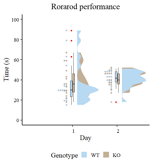
Let’s check out the preliminary view of the info utilizing rain cloud plot as proven in Dr. Guilherme A. Franchi in this Nice weblog submit.
edv <- ggplot(information, aes(x = Day, y = Trial3, fill=Genotype)) +
scale_fill_ghibli_d("SpiritedMedium", route = -1) +
geom_boxplot(width = 0.1,
outlier.colour = "purple") +
xlab('Day') +
ylab('Time (s)') +
ggtitle("Rorarod efficiency") +
theme_classic(base_size=18, base_family="serif")+
theme(textual content = element_text(dimension=18),
axis.textual content.x = element_text(angle=0, hjust=.1, vjust = 0.5, colour = "black"),
axis.textual content.y = element_text(colour = "black"),
plot.title = element_text(hjust = 0.5),
plot.subtitle = element_text(hjust = 0.5),
legend.place="backside")+
scale_y_continuous(breaks = seq(0, 100, by=20),
limits=c(0,100)) +
# Line beneath provides dot plots from {ggdist} package deal
stat_dots(facet = "left",
justification = 1.12,
binwidth = 1.9) +
# Line beneath provides half-violin from {ggdist} package deal
stat_halfeye(alter = .5,
width = .6,
justification = -.2,
.width = 0,
point_colour = NA)
edv

Figure 2 appears totally different than the unique Dr. Guilherme A. Franchi It’s because you’re plotting two components as a substitute of 1. Nevertheless, the character of the plot is identical. Discover the purple dot. These are what could be thought-about excessive observations that tip the measure of central tendency (particularly the imply) in a single route. It has additionally been noticed that the variances are totally different, so modeling sigma offers a greater estimate. The duty right here is to mannequin the output utilizing brms package deal.
