


Intentionally Exploring Design Selections for Parameter Environment friendly Finetuning (PEFT) with LoRA
Excellent news: Utilizing LoRA for Parameter Environment friendly Finetuning (PEFT) may be simple. With a easy technique of adapting all linear modules and a few gentle tuning of the training price, you may obtain good efficiency. You possibly can cease studying right here!
However what in order for you extra? What in case you’re searching for a deeper understanding of which modules to tune, and optimize your mannequin for efficiency, GPU reminiscence utilization or coaching pace? When you’re searching for a extra nuanced understanding and management over these points, then you definately’re in the fitting place.
Be a part of me on this journey as we navigate the winding street to parameter effectivity. We’ll delve into the deliberate design choices that may enable you to get probably the most out of LoRA whereas providing you extra management and a greater understanding of your mannequin’s efficiency. Let’s embark on this thrilling exploration collectively.
You’d get probably the most out of this text if you have already got a minimum of a primary understanding of LoRA, like what we coated within the earlier article. Moreover we’re optimizing a RoBERTa mannequin [1], which makes use of the transformer architecture. A common understanding of the essential parts helps, however is just not completely essential to observe alongside on the primary topic.
Within the earlier article, we explored apply LoRA to coach adapters that solely require a fraction of the parameters wanted for a full finetuning. We additionally noticed how such an implementation may seem like in code. Nevertheless, our focus was totally on the mechanical points. We didn’t handle which modules to adapt, nor dimension the adapters for effectivity and efficiency.
Immediately, that is our focus.
We zoom out and acknowledge that there are numerous algorithmic design choices that we now have to make, lots of which affect one another. These are sometimes expressed as hyperparameters by the unique algorithm creators. To deal with the sheer variety of potential combos of hyperparameters and their values we’ll use a scientific method to study concerning the relative impression; of those design choices. Our goal is just not solely to ultimately obtain good efficiency for our mannequin at hand, however we additionally wish to run experiments to collect empirical suggestions to strengthen our intuitive understanding of the mannequin and its design. This is not going to solely serve us nicely for as we speak’s mannequin, job, and dataset, however a lot of what we study will probably be transferable. It would give us better confidence shifting ahead as we work on variations of the mannequin, new duties, and datasets within the future.
Execution of Experiments:
I will probably be utilizing Amazon SageMaker Computerized Mannequin Tuning (AMT) to run the experiments all through this text. With AMT I’ll both intentionally discover and analyze the search area, or, routinely discover a good mixture of hyperparameter values.
As a aspect observe, ‘tuning’ is a time period that serves two functions on this article. On one hand, we use ‘hyperparameter tuning’ to discuss with the adjustment of hyperparameter values in mannequin coaching, a course of automated by SageMaker’s Computerized Mannequin Tuning. However, we use ‘tuning’ to explain the method of beginning with a pre-trained mannequin after which finetuning its parameters (not the hyperparameters) for our particular downstream job.
To keep up focus, I’ll preserve the implementation particulars on this article transient. Nevertheless, one can find all of the experiments with all their particulars within the linked notebooks.
I additionally encourage you to study extra background about utilizing AMT, the variations between the search methods Random Search and Bayesian Optimization, the idea of heat beginning tuning jobs and about visualizing/analyzing the outcomes. All of which, are mentioned in this article:
Baselines: What to match to?
We are going to give attention to architectural choices:
- Which modules ought to we adapt?
- On what layers? All of them? Some? Simply the center layers?
- How massive ought to the module adapters be? What ought to r, the rank of the LoRA matrices, be?
Nevertheless, earlier than we begin experimenting, how can we be sure that we’re heading in the right direction and that our modifications have a constructive impression? Let’s outline some baselines to match our progress to.
If discovering baselines for comparability doesn’t attraction to you, be happy to skip forward to the subsequent part “What to tune?”.
Over time, we hope to watch that our coaching runs are producing higher outcomes. However when are we finished and may cease experimenting?
Seeing no additional enhancements after some time might point out that we now have achieved the optimum. Nevertheless, it might additionally imply that we now have ran out of concepts to check out, regardless that extra was potential.
Efficiency Expectations and Reproducibility
With a purpose to interpret the outcomes of our experiments, we have to set up clear efficiency expectations for our mannequin. This consists of an understanding of the perfect efficiency as an higher certain, in addition to the minimal efficiency we anticipate to see.
Deep studying is inherently noisy, which means that no two runs will produce the very same consequence. This raises vital questions concerning the outcomes we observe. Is the efficiency we’re seeing reproducible utilizing the hyperparameter values we examined with, or did we simply get fortunate with this specific run? To reply these questions, we have to validate a set of hyperparameter values that we’ve discovered to carry out nicely. On this article I’ll do that by working the identical hyperparameter values 5 occasions to calculate the imply efficiency and its variance.
Anticipated efficiency — Full Finetuning: In our case reasoning concerning the anticipated efficiency is straightforward. We’re finetuning a sentiment evaluation job on the sst-2 dataset utilizing the RoBERTa base mannequin, as was finished within the RoBERTa paper [1].
Due to this fact, we will straight use the numbers reported by the authors as a sanity verify. We are going to align our setup and the hyperparameters used with these within the paper.
We nonetheless run the coaching ourselves, in order that we now have a verified setup and coaching process earlier than we apply LoRA to it. Consequently, we will carry out a sanity verify to make sure that the numbers we observe roughly match these from the paper. If we can’t match the numbers, we would wish to verify our setup.
The RoBERTa paper [1] reported an accuracy of 94.8in desk 8. This serves as our benchmark for anticipated efficiency throughout full fine-tuning. After checking that we’re within the ball park of that quantity, we are going to use our personal setup and the outcomes as a baseline for evaluating all the next experiments, that are derived from our setup.
Anticipated efficiency — LoRA Finetuning: That is straightforward as nicely. The promise of LoRA is to virtually match the total finetuning efficiency, however with solely a fraction of the parameters of a full finetuning.
Therefore, we are going to evaluate to our outcomes from the total finetuning efficiency as described within the previous part.
Anticipated minimal efficiency: One potential baseline can be random efficiency. For our job with two courses that will be 0.5. However we aren’t constructing a mannequin from scratch and from the papers we already know that the LoRA method is working very nicely, so random efficiency wouldn’t be an informative baseline.
As an alternative, let’s use a baseline the place we solely prepare the classifier and preserve the embeddings and transformer layers frozen, within the state they got here from the pre-training. This could lead to a a lot decrease efficiency than a full finetuning, however a lot better than random, although. Importantly, it must also function a comparability level to motive about non-functional points like parameter effectivity, reminiscence utilization, and coaching throughput.
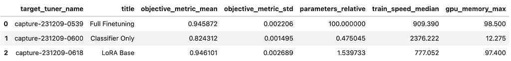
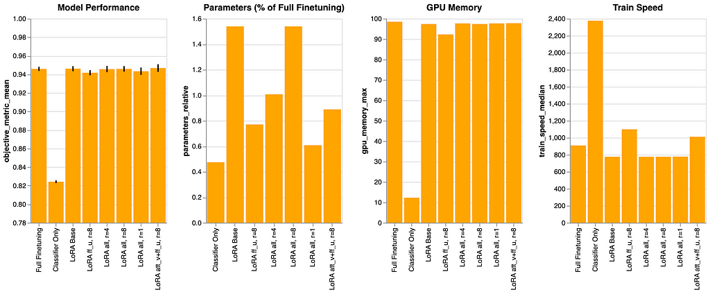
All situations above have been run 5 occasions, and the imply efficiency is proven within the diagram. You may also deduce that we’re within the ballpark of the efficiency from the RoBERTa paper with the situations “Full Finetuning”. As we hoped for, “LoRA Base” (adapting all linear modules) matches that efficiency, however makes use of fewer parameters. The state of affairs “Classifier Solely” performs a lot worse, as anticipated, however is cheaper when it comes to parameters and trains quicker.
Shifting ahead, we are going to now take our numbers as baselines to match future experiments to.
You could find extra particulars within the accompanying notebook.
Execution of Experiments:
First, for every baseline, we seek for an optimum studying price parameter worth. We use Bayesian Optimization to effectively discover after which exploit the search area.
Second, the perfect hyperparameter values we discovered for a state of affairs could or could not essentially reproduce good outcomes. It may very well be that the hyperparameter values we recognized are solely the perfect relative to the opposite values we explored. Possibly the values we discovered weren’t related in any respect, e.g. the mannequin was not delicate on this worth vary? To estimate how good the findings maintain up, for every state of affairs, we run the perfect mixture of hyperparameter values once more 5 occasions and report the noticed normal deviation on the target metric.
LoRA Base Situation — First End result: It’s encouraging to see that the LoRA finetuning method, state of affairs “LoRA Base”, is already acting on par with “Full Finetuning”, regardless of it simply utilizing ~1% of the parameters. Moreover, on this method we’re adapting all linear modules with the identical adapter dimension (r=8). This can be a easy place to begin that apparently produces good efficiency regardless of its simplicity.
Secondary Hyperparameters: As a degree of observe, we primarily seek for good values for the hyperparameter r and the modules we wish to adapt. To maintain issues easy, we solely tune only a few further hyperparameters. For the baselines it’s simply the training price and the variety of epochs. We use Bayesian Optimization because the search technique utilizing Amazon SageMaker Computerized Mannequin Tuning (AMT).
We observe steerage from the referenced papers on setting different hyperparameters, reminiscent of weight decay and dropout. We preserve these hyperparameters mounted all through the article, in order that we will isolate the impression of the hyperparameters that outline the LoRA structure, making it simpler to see how our most important hyperparameters affect efficiency.
Do you, expensive reader, plan to repeat the steps from this text? Are you aiming to seek out the perfect hyperparameters in your personal mannequin, job, and dataset that you simply intend to make use of in manufacturing? In that case, it will make sense to additionally embody the secondary hyperparameters. Ideally, you need to do that in the direction of the tip of your exploration and tuning effort — when you could have already considerably narrowed the search scope — after which goal to additional enhance efficiency, even when simply barely.
Hyperparameters: What to tune?
Let’s get began with our most important exercise.
The design choices left for us within the mannequin structure are sometimes expressed as hyperparameters. For LoRA particularly, we will outline which modules to adapt and how massive r needs to be for every module’s adapter.
Within the final article we solely advised deciding on these modules primarily based on our understanding of the duty and the structure.
Now, we’ll dive deeper. The place ought to we apply finetuning at all?
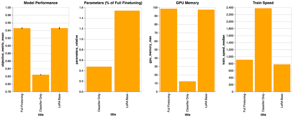
Within the illustration above, you may see all of the potential modules that we might finetune–together with the classifier and the embeddings–on the left. On the fitting, I’ve made a pattern choice for the illustration . However how will we arrive at an precise choice?
Let’s take a look at our choices from a excessive degree:
- Classifier
It’s clear that we completely want to coach the classifier. It is because it has not been skilled throughout pre-training and, therefore, for our finetuning, it’s randomly initialized. Moreover, its central place makes it extremely impactful on the mannequin efficiency, as all data should stream by it. It additionally has probably the most rapid impression on the loss calculation because it begins on the classifier. Lastly, it has few parameters, subsequently, it’s environment friendly to coach.
In conclusion, we at all times finetune the classifier, however don’t adapt it (with LoRA). - Embeddings
The embeddings reside on the backside–near the inputs–and carry the semantic which means of the tokens. That is vital for our downstream job. Nevertheless, it’s not “empty”. Even with out finetuning, we might get all of what was realized throughout pre-training. At this level, we’re contemplating whether or not finetuning the embeddings straight would give us further skills and if our downstream job would profit from a refined understanding of the token meanings?
Let’s mirror. If this had been the case, might this extra data not even be realized in one of many layers above the embeddings, maybe much more effectively?
Lastly, the embeddings sometimes have a lot of parameters, so we must adapt them earlier than finetuning.
Taking each points collectively, we determined to go on this selection and never make the embeddings trainable (and consequently not apply LoRA to them). - Transformer Layers
Finetuning all parameters within the transformer layers can be inefficient. Due to this fact, we have to a minimum of adapt them with LoRA to develop into parameter-efficient. This leads us to contemplate whether or not we must always prepare all layers, and all parts inside every layer? Or ought to we prepare some layers, some parts, or particular combos of each?
There isn’t a common reply right here. We’ll adapt these layers and their modules and discover the main points additional on this article.
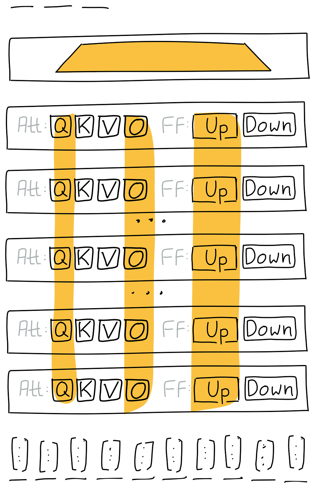
Within the illustration above, on the fitting, you may see an exemplary choice of modules to finetune on the fitting. This is only one mixture, however many different combos are potential. Consider as nicely that the illustration solely reveals 5 layers, whereas your mannequin probably has extra. For example, the RoBERTa base mannequin–utilized in our instance–has 12 layers, a quantity that’s thought of small by as we speak’s requirements. Every layer additionally has 6 parts:
- Consideration: Question, Key, Worth, Output
- Feed Ahead: Up, Down
Even when we disregard that we additionally wish to tune r and — for now — simply give attention to the binary determination of which modules to incorporate, it will depart us with 64 (2**6) combos per layer. Given this solely appears to be like on the combos of 1 layer, however that we now have 12 layers that may be mixed, we find yourself with greater than a sextillion combos:
In [1]: (2**6)**12.
Out[1]: 4.722366482869645e+21
It’s straightforward to see that we can’t exhaustively compute all combos, not to mention to discover the area manually.
Usually in laptop science, we flip to the cube after we wish to discover an area that’s too massive to completely examine. However on this case, we might pattern from that area, however how would we interpret the outcomes? We might get again quite a few arbitrary mixture of layers and parts (a minimum of 12*6=72 following the small instance of above). How would we generalize from these particulars to seek out higher-level guidelines that align with our pure understanding of the issue area? We have to align these particulars with our conceptual understanding on a extra summary degree.
Therefore, we have to take into account teams of modules and search for buildings or patterns that we will use in our experiments, somewhat than working on a set of particular person parts or layers. We have to develop an instinct about how issues ought to work, after which formulate and take a look at hypotheses.
Query: Does it assist to experiment on outlined teams of parameters in isolation? The reply is sure. These remoted teams of parameters can paved the way regardless that we might have to mix a few of them later to attain the perfect outcomes. Testing in isolation permits us to see patterns of impression extra clearly.
Nevertheless, there’s a danger. When these patterns are utilized in mixture, their impression could change. That’s not good, however let’s not be so detrimental about it 🙂 We have to begin someplace, after which refine our method if wanted.
Prepared? Let’s do that out.
Tuning Vertically / Layer-wise
I believe that the higher layers, nearer to the classification head, will probably be extra impactful than the decrease layers. Right here is my pondering: Our job is sentiment evaluation. It will make sense, wouldn’t it, that many of the particular choices must be made both within the classification head or near it? Like recognizing sure phrases (“I wanted that like a gap in my head”) or composed constructs (“The check-in expertise negated the in any other case great service”). This might recommend that it’s essential to finetune the parameters of our community that outline how completely different tokens are used collectively–in context–to create a sentiment versus altering the which means of phrases (within the embeddings) in comparison with their which means throughout the pre-training.
Even when that’s not at all times the case, adapting the higher layers nonetheless offers the chance to override or refine choices from the decrease layers and the embeddings. However, this implies that finetuning the decrease layers is much less vital.
That sounds like a strong speculation to check out (Oops. Message from future Mariano: Don’t cease studying right here).
As an apart, we aren’t reflecting on the overall necessity of the embeddings or any of the transformer layers. That call has already been made: all of them had been a part of the pre-training and will probably be a part of our finetuned mannequin. What we’re contemplating at this level is how we will finest assist the mannequin study our downstream job, which is sentiment evaluation. The query we’re asking is: which weights ought to we finetune for impression and to attain parameter effectivity?
Let’s put this to the take a look at.
To obviously see the impact of our speculation, what will we take a look at it towards? Let’s design experiments that ought to exaggerate the impact:
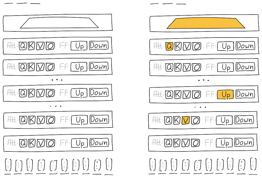
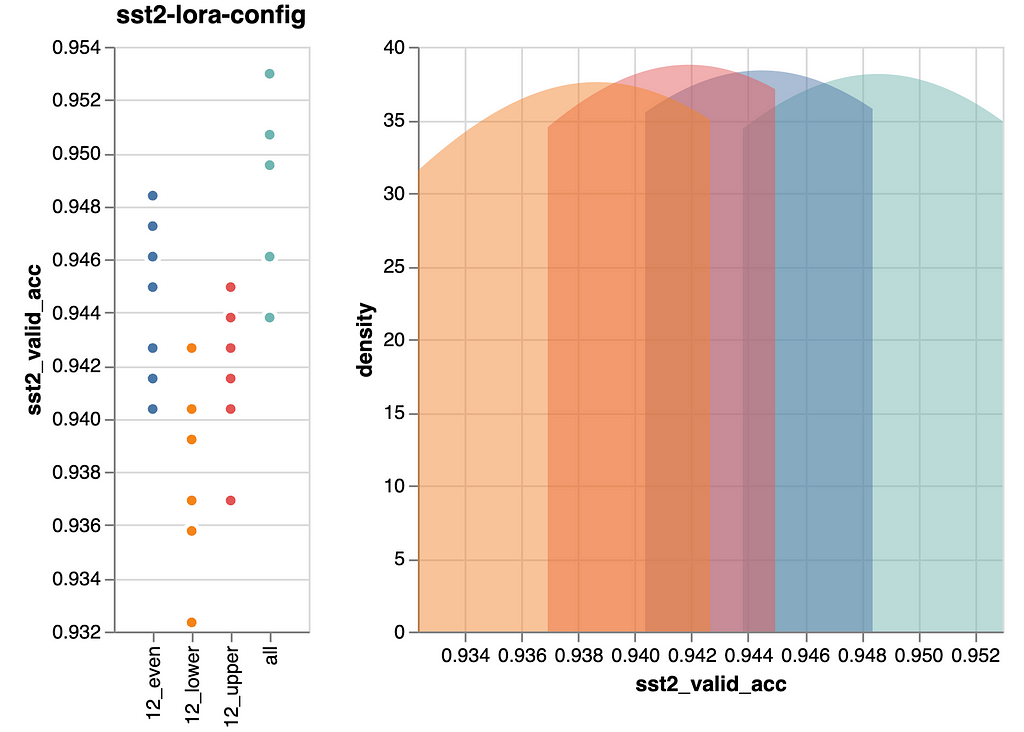
- In our first experiment we finetune and adapt all parts of the higher half of the mannequin, specifically layers 7–12 in our instance. That is our speculation.
- In distinction, we run one other experiment the place we solely finetune the layers within the decrease half of the mannequin. Particularly, we prepare layers 1–6 with all parts. That’s the other of our speculation.
- Let’s take into account one other contrastive speculation as nicely: {that a} gentle contact to all layers is extra useful than simply tuning the highest layers. So, let’s additionally embody a 3rd state of affairs the place we finetune half of the layers however unfold them out evenly.
- Let’s additionally embody an experiment the place we tune all layers (not depicted within the illustration above). This isn’t a good efficiency comparability as we prepare twice as many parameters as within the first three experiments. Nevertheless, for that motive, it highlights how a lot efficiency we probably lose within the earlier situations the place we had been tuning solely half the variety of parameters.
In abstract, we now have 3+1 situations that we wish to run as experiments. Listed below are the outcomes:
Execution of Experiments:
We begin by utilizing the already tuned studying price, epochs. Then, we run trials (coaching runs) with completely different values for the state of affairs settings, reminiscent of decrease, higher, even, all. Inside AMT, we run these experiments as a Grid Search.
Query: Grid Search is thought to be easy, however inefficient to find the perfect answer. So why are we utilizing it?
Let’s take a step again. If we had been to run just a few trials with Bayesian Search, we’d shortly study hyperparameter values which can be performing nicely. This might bias the next trials to give attention to these values, i.e., pre-dominantly keep nearer to identified good values. Whereas more and more exploiting what we study concerning the search area is an efficient technique to seek out the perfect values, its bias makes it obscure the explored area, as we under-sample in areas that confirmed low efficiency early on.
With Grid Search, we will exactly outline which parameter values to discover, making the outcomes simpler to interpret.
In reality, in case you had been to take a look at the supplied code, you’d see that AMT would reject sampling the identical values greater than as soon as. However we would like that, therefore, we introduce a dummy variable with values from 0 to the variety of trials we wish to conduct. That is useful, permitting us to repeat the trials with the identical hyperparameter values to estimate the usual deviation of this mixture.
Whereas we used 5 trials every for an already tuned baseline state of affairs above to see how nicely we will reproduce a selected mixture of hyperparameter values, right here we use 7 trials per mixture to get a barely extra exact understanding of this mixture’s variance to see tiny variations.
The identical ideas are utilized to the next two situations on this article and won’t be talked about once more henceforth.
Let’s get the straightforward factor out of the way in which first: As anticipated, tuning all layers and consequently utilizing double the variety of parameters, improves efficiency probably the most. This enchancment is obvious within the backside determine.
Additionally, the peaks of all situations, as proven within the density plots on the fitting of the person figures, are comparatively shut. When evaluating these peaks, which signify probably the most ceaselessly noticed efficiency, we solely see an enchancment of ~0.08 in validation accuracy between the worst and finest state of affairs. That’s not a lot. Due to this fact, we take into account it a wash.
Regardless, let’s nonetheless study our authentic speculation: We (me, actually) anticipated that finetuning the higher six layers would yield higher efficiency than finetuning the decrease six layers. Nevertheless, the info disagrees. For this job it makes no distinction. Therefore, I must replace my understanding.
We’ve got two potential takeaways:
- Spreading the layers evenly is somewhat higher than specializing in the highest or backside layers. That stated, the development is so small that this perception could also be brittle and may not generalize nicely, not occasion to new runs of the identical mannequin. Therefore, we are going to discard our “discovery”.
- Tuning all layers, with double the price, produces marginally higher outcomes. This final result, nonetheless, is no surprise anybody. Nonetheless good to see confirmed although, as we in any other case would have discovered a possibility to avoid wasting trainable parameters, i.e., value.
Total, good to know all of that, however as we don’t take into account it actionable, we’re shifting on. If you’re , yow will discover extra particulars on this notebook.
Tuning Horizontally / Element-wise
Inside every transformer layer, we now have 4 realized projections used for consideration that may be tailored throughout finetuning:
- Q — Question, 768 -> 768
- Ok — Key, 768 -> 768
- V — Worth, 768 -> 768
- O — Output, 768 -> 768
Along with these, we use two linear modules in every position-wise feedforward layer that reside inside the similar transformer layer because the projections from above:
- Up — Up projection, 768 -> 3072
- Down — Down projection, 3072 -> 768
We will already see from the numbers above that the feedforward layers (ff) are 4 occasions as massive because the QKVO projections we beforehand mentioned. Therefore the ff parts could have a probably bigger impression and definitely larger value.
Apart from this, what different expectations might we now have? It’s onerous to say. We all know from Multi-Question Consideration [3] that the question projection is especially vital, however does this significance maintain when finetuning with an adapter on our job (versus, for instance, pre-training)? As an alternative, let’s check out what the impression of the person parts is and proceed primarily based on these outcomes. We will see which parts are the strongest and possibly it will permit us to simply choose these for tuning going ahead.
Let’s run these experiments and examine the outcomes:
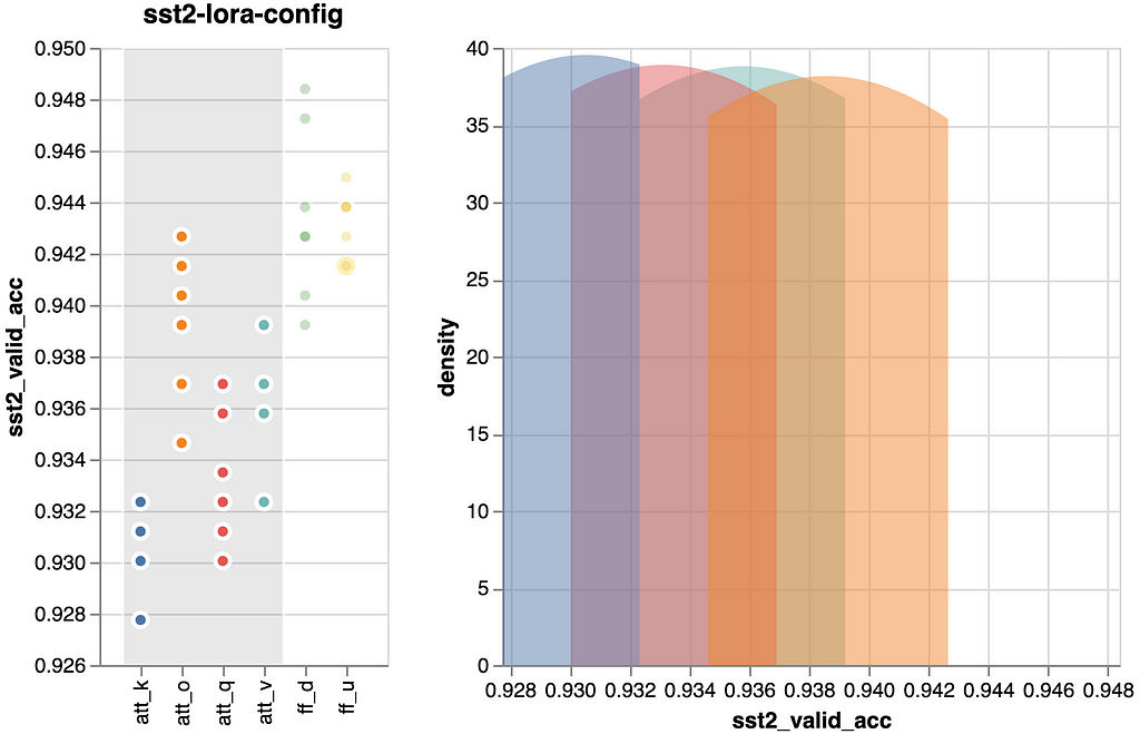
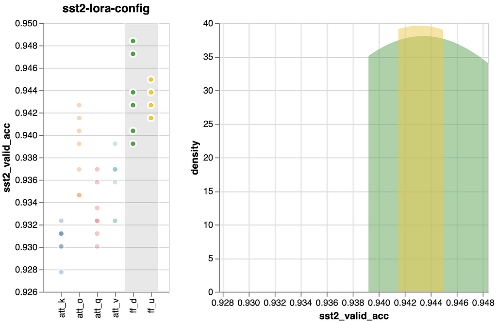
As was to be anticipated, the ff layers use their four-times dimension benefit to outperform the eye projections. Nonetheless, we will see that there are variations inside these two teams. These variations are comparatively minor, and if you wish to leverage them, it’s essential to validate their applicability in your particular job.
An vital statement is that by merely tuning one of many ff layers (~0.943), we might virtually obtain the efficiency of tuning all modules from the “LoRA Base” state of affairs (~0.946). Consequently, if we’re seeking to steadiness between general efficiency and the parameter rely, this may very well be technique. We’ll preserve this in thoughts for the ultimate comparability.
Inside the consideration projections (center determine) it seems that the question projection didn’t show as impactful as anticipated. Contrarily, the output and worth projections proved extra helpful. Nevertheless, on their very own, they weren’t that spectacular.
Thus far, we now have appeared on the particular person contributions of the parts. Let’s additionally verify if their impression overlaps or if combining parts can enhance the outcomes.
Let’s run among the potential combos and see if that is informative. Listed below are the outcomes:
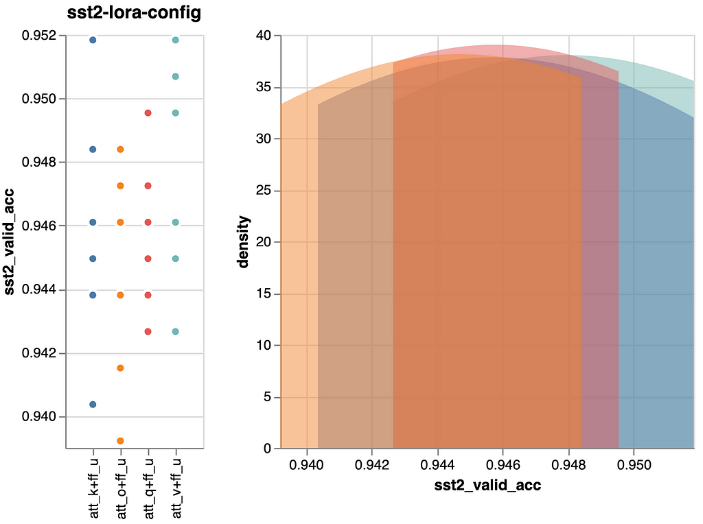
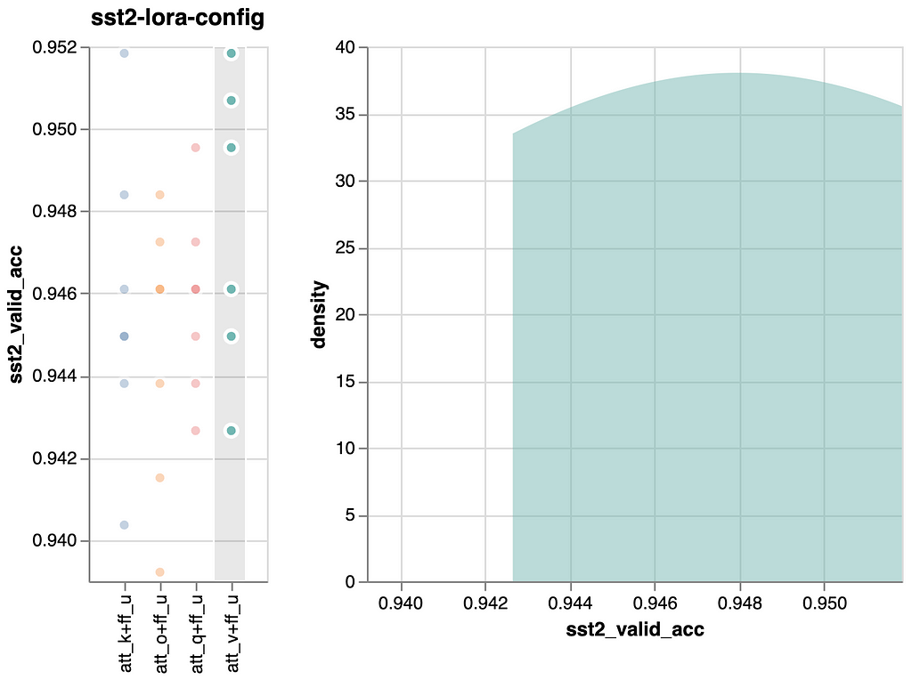
Trying on the numbers charted above the primary takeaway is that we now have no efficiency regressions. Provided that we added extra parameters and mixed present combos, that’s the way it needs to be. However, there may be at all times the possibility that when combining design choices their mixed efficiency is worse than their particular person efficiency. Not right here although, good!
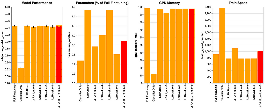
We should always not over-interpret the outcomes, however it’s fascinating to acknowledge that after we testing our speculation individually the output projection’s efficiency was barely forward of the efficiency of the worth projection. Right here now, together with the position-wise feed ahead up projection this relationship is reversed (now: o+up ~0.945, v+up ~0.948).
We’ll additionally acknowledge within the earlier experiment, that the up projection was already performing virtually on that degree by itself. Due to this fact, we preserve our enthusiasm in verify, however embody this state of affairs in our ultimate comparability. If solely, as a result of we get a efficiency that’s barely higher than when tuning and adapting all parts in all layers, “LoRA Base”, however with a lot fewer parameters.
You could find extra particulars on this notebook.
Tuning r
We all know from the literature [2] that it is strongly recommended to make use of a small r worth, which means that r is simply a fraction of the minimal dimension of the unique module, e.g. to make use of 8 as a substitute of 768. Nevertheless, let’s validate this for ourselves and get some empirical suggestions. Might or not it’s value investigating utilizing a bigger worth for r, regardless of the standard knowledge?
For the earlier trials, we used r=8 and invested extra time to tune learning-rate and the variety of epochs to coach for this worth. Now attempting completely different values for r will considerably alter the capability of the linear modules. Ideally, we might re-tune the learning-rate for every worth of r, however we goal to be frugal. Consequently, for now, we persist with the identical learning-rate. Nevertheless, as farther we go away from our tuned r=8value as stronger the necessity to retune the opposite hyperparameters talked about above.
A consideration we have to keep in mind when reviewing the outcomes:
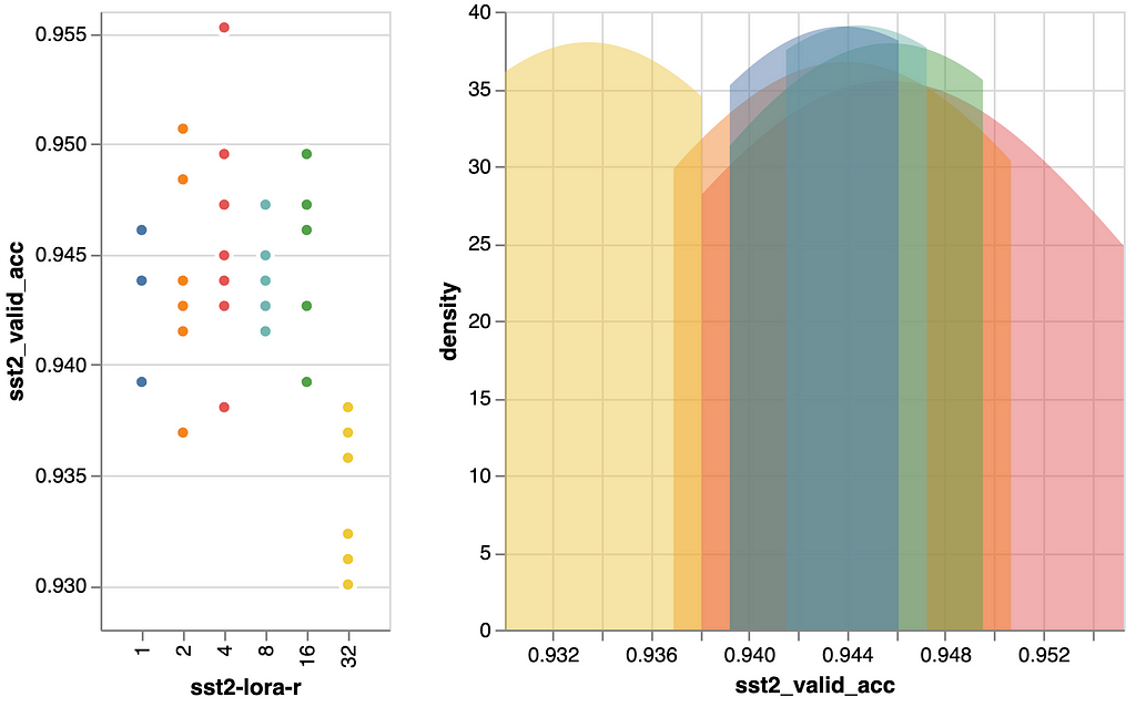
Within the first determine, we see that the mannequin efficiency is just not notably delicate to further capability with good performances at r=4 and r=8. r=16was a tiny bit higher, however can be dearer when it comes to parameter rely. So let’s preserve r=4 and r=8 in thoughts for our ultimate comparability.
To see the impact of r on the parameter rely, we may even embody r=1 within the ultimate comparability.
One odd factor to watch within the figures above is that the efficiency is falling off sharply at r=32. Offering a mannequin, that makes use of residual connections, extra capability ought to yield the identical or higher efficiency than with a decrease capability. That is clearly not the case right here. However as we tuned the learning-rate for r=8 and we now have many extra learnable parameters with r=32 (see the higher proper panel in previous determine) we must also scale back the learning-rate, or ideally, re-tune the learning-rate and variety of epochs to adapt to the a lot bigger capability. Trying on the decrease proper panel within the earlier determine we must always then additionally take into account including extra regularization to cope with the extra pronounced overfitting we see.
Regardless of the overall potential for enchancment when offering the mannequin with extra capability, the opposite values of r we noticed didn’t point out that extra capability would enhance efficiency with out additionally markedly rising the variety of parameters. Due to this fact, we’ll skip chasing a fair bigger r.
Extra particulars on this notebook.
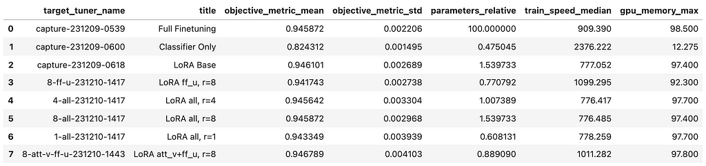
Remaining Comparability
All through this lengthy article, we now have gathered quite a few analytical outcomes. To consolidate these findings, let’s discover and evaluate a number of fascinating combos of hyperparameter values in a single place. For our functions, a result’s thought of fascinating if it both improves the general efficiency of the mannequin or provides us further insights about how the mannequin works to in the end strengthen our intuitive understanding
All experiments finetune the sst2 job on RoBERTa base as seen within the RoBERTa paper [1].
Execution of Experiments:
As earlier than, after I present the outcomes of a state of affairs (reported because the “target_tuner_name” column within the desk above, and as labels on the y-axis within the graph), it’s primarily based on executing the similar mixture of hyperparameter values 5 occasions. This permits me to report the imply and normal deviation of the target metric.
Now, let’s focus on some observations from the situations depicted within the graph above.
Classifier Solely
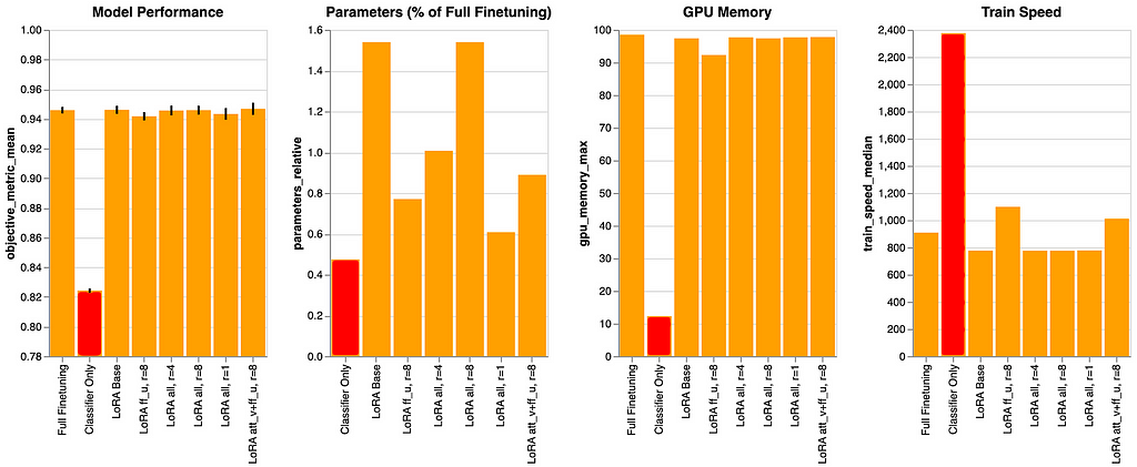
This baseline—the place we solely prepare the classifier head—has the bottom value. Consult with parameters_relative, which signifies the share of parameters wanted, in comparison with a full finetuning. That is illustrated within the second panel, displaying that ~0.5% is the bottom parameter rely of all situations.
This has a useful impression on the “GPU Reminiscence” panel (the place decrease is best) and markedly within the “Practice Pace” panel (the place larger is best). The latter signifies that this state of affairs is the quickest to coach, due to the decrease parameter rely, and likewise as a result of there are fewer modules to deal with, as we don’t add further modules on this state of affairs.
This serves as an informative bare-bones baseline to see relative enhancements in coaching pace and GPU reminiscence use, but in addition highlights a tradeoff: the mannequin efficiency (first panel) is the bottom by a large margin.
Moreover, this state of affairs reveals that 0.48% of the total fine-tuning parameters signify the minimal parameter rely. We allocate that fraction of the parameters solely for the classifier. Moreover, as all different situations tune the classifier, we constantly embody that 0.48% along with no matter parameters are additional tuned in these situations.
LoRA Base
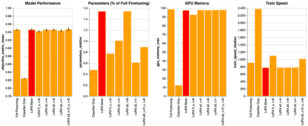
This state of affairs serves as the muse for all experiments past the baselines. We person=8 and adapt and finetune all linear modules throughout all layers.
We will observe that the mannequin efficiency matches the total finetuning efficiency. We would have been fortunate on this case, however the literature recommend that we will anticipate to almost match the total finetuning efficiency with nearly 1% of the parameters. We will see proof of this right here.
Moreover, due to adapting all linear modules, we see that the prepare pace is the bottom of all experiments and the GPU reminiscence utilization is amongst the best, however in step with many of the different situations.
LoRA all, r={1,4,8}
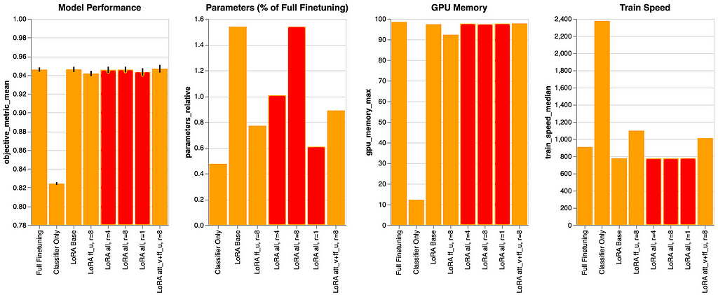
Total, these situations are variations of “LoRA Base” however with completely different values of r. There may be solely a small distinction within the efficiency. Nevertheless, as anticipated, there’s a constructive correlation between r and the parameter rely and a barely constructive correlation between r and GPU reminiscence utilization. Regardless of the latter, the worth of r stays so low that this doesn’t have a considerable impression on the underside line, particularly the GPU reminiscence utilization. This confirms what we explored within the authentic experiments, component-wise, as mentioned above.
When reviewing r=1, nonetheless, we see that it is a particular case. With 0.61% for the relative parameter rely, we’re only a smidgen above the 0.48% of the “Classifier Solely” state of affairs. However we see a validation accuracy of ~0.94 with r=1, in comparison with ~0.82 with “Classifier Solely”. With simply 0.13% of the entire parameters, tailored solely within the transformer layers, we will elevate the mannequin’s validation accuracy by ~0.12. Bam! That is spectacular, and therefore, if we’re fascinated with a low parameter rely, this may very well be our winner.
Relating to GPU reminiscence utilization, we’ll evaluate this a bit later. However briefly, moreover allocating reminiscence for every parameter within the mannequin, the optimizer, and the gradients, we additionally must preserve the activations round to calculate the gradients throughout backpropagation.
Moreover, bigger fashions will present a much bigger impression of selecting a small worth for r.
For what it’s value, the state of affairs “LoRA all, r=8” used equivalent hyperparameter values to “LoRA Base”, however was executed independently. To make it simpler to match r=1, r=4 and r=8, this state of affairs was nonetheless evaluated.
LoRA ff_u
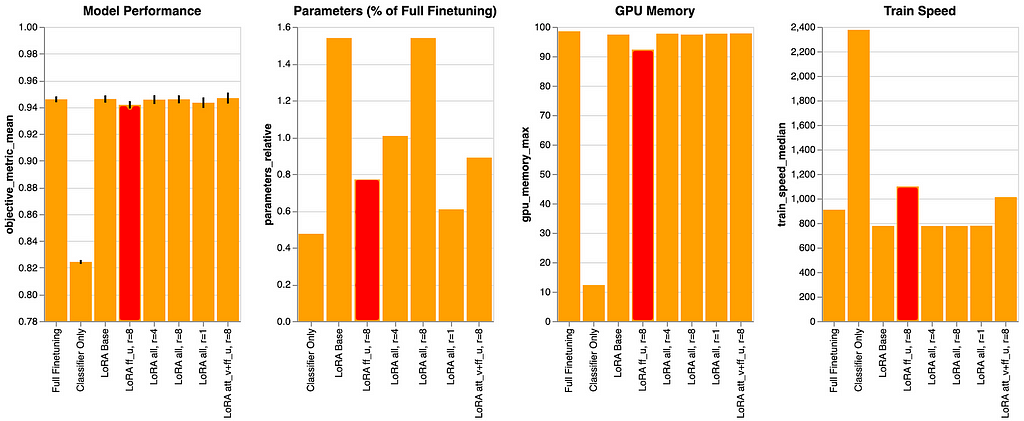
On this state of affairs we’re tuning solely the position-wise feed ahead up projections, throughout all layers. This results in a discount in each the variety of parameters and the variety of modules to adapt. Consequently, the info reveals an enchancment in coaching pace and a discount in GPU reminiscence utilization.
However we additionally see a small efficiency hit. For “LoRA Base” we noticed ~0.946, whereas on this state of affairs we solely see ~0.942, a drop of ~0.04.
Particulars on the comparisons on this notebook.
Sidestep: GPU Reminiscence / Gradient Checkpointing
When wanting on the GPU reminiscence panel above, two issues develop into apparent:
One — LoRA, by itself, doesn’t dramatically scale back the reminiscence footprint
That is very true when we adapt small fashions like RoBERTa base with its 125M parameters.
Within the earlier article’s part on intrinsic dimensionality, we realized that for present era fashions (e.g., with 7B parameters), absolutely the worth of r may be even smaller than for smaller capability fashions. Therefore, the memory-saving impact will develop into extra pronounced with bigger fashions.
Moreover utilizing LoRA makes utilizing quantization simpler and extra environment friendly – an ideal match. With LoRA, solely a small share of parameters have to be processed with excessive precision: It is because we replace the parameters of the adapters, not the weights of the unique modules. Therefore, nearly all of the mannequin weights may be quantized and used at a lot decrease precision.
Moreover, we sometimes use AdamW as our optimizer. In contrast to SGD, which tracks solely a single world studying price, AdamW tracks shifting averages of each the gradients and the squares of the gradients for every parameter. This means that for every trainable parameter, we have to preserve monitor of two values, which might probably be in FP32. This course of may be fairly expensive. Nevertheless, as described within the earlier paragraph, when utilizing LoRA, we solely have just a few parameters which can be trainable. This may considerably scale back the price, in order that we will use the sometimes parameter-intensive AdamW, even with massive r values.
We could look into these points partially 4 of our article collection, given sufficient curiosity of you, expensive reader.
Two–GPU reminiscence utilization is simply not directly correlated with parameter rely
Wouldn’t or not it’s nice if there was a direct linear relationship between the parameter rely and the wanted GPU reminiscence? Sadly there are a number of findings within the diagrams above that illustrate that it isn’t that straightforward. Let’s discover out why.
First we have to allocate reminiscence for the mannequin itself, i.e., storing all parameters. Then, for the trainable parameters, we additionally must retailer the optimizer state and gradients (for every trainable parameter individually). As well as we have to take into account reminiscence for the activations, which not solely is determined by the parameters and layers of the mannequin, but in addition on the enter sequence size. Plus, it’s essential to do not forget that we have to preserve these activations from the ahead go with the intention to apply the chain rule throughout the backward go to do backpropagation.
If, throughout backpropagation, we had been to re-calculate the activations for every layer when calculating the gradients for that layer, we might not preserve the activations for thus lang and will save reminiscence at the price of elevated computation.
This method is called gradient checkpointing. The quantity of reminiscence that may be saved is determined by how a lot further reminiscence for activations must be retained. It’s vital to do not forget that backpropagation entails repeatedly making use of the chain rule, step-by-step, layer by layer:
Recap — Chain Rule throughout Again Propagation
Throughout backpropagation, we calculate the error on the prime of the community (within the classifier) after which propagate the error again to all trainable parameters that had been concerned. These parameters are adjusted primarily based on their contributions to the error, to do higher sooner or later. We calculate the parameters’ contributions by repeatedly making use of the chain rule, begin on the prime and traversing the computation graph in the direction of the inputs. That is essential as a result of any change in a parameter on a decrease layer can probably impression the parameters in all of the layers above.
To calculate the native gradients (for every step), we might have the values of the activations for all of the steps between the respective trainable parameter and the highest (the loss operate which is utilized on the classification head). Thus, if we now have a parameter in one of many prime layers (near the pinnacle), we have to preserve fewer activations in comparison with when coaching a parameter within the decrease layers. For these decrease layer parameters, we have to traverse a for much longer graph to achieve the classification head and, therefore, want to keep up extra reminiscence to maintain the activations round.
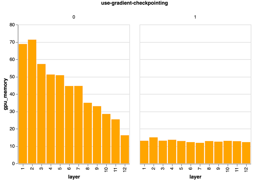
In our particular mannequin and job, you may see the impact illustrated beneath. We prepare a person mannequin for every layer, wherein solely that individual layer undergoes coaching. This manner, we will isolate the impact of the layer’s relative place. We then plot the quantity of GPU reminiscence required for every mannequin, and subsequently for every layer, throughout coaching.
Within the graph beneath (see left panel) you may see that if we’re nearer to the underside of the mannequin (i.e., low layer quantity) the GPU reminiscence requirement is decrease than if we’re near the highest of the mannequin (i.e., excessive layer quantity) the place the loss originates.
With gradient checkpointing enabled (see proper panel), we not can acknowledge this impact. As an alternative of saving the activations till backprop we re-calculate them when wanted. Therefore, the distinction in reminiscence utilization between the left and proper panel are the activations that we preserve for the backward go.
Execution of Experiments:
As with earlier experiments, I used AMT with Grid Search to offer unbiased outcomes.
It is very important keep in mind, that recalculating the activations throughout backpropagation is gradual, so we’re buying and selling of computational pace with reminiscence utilization.
Extra particulars on the testing may be discovered on this notebook.
As an apart, to the perfect of my understanding, utilizing Gradient Checkpointing ought to solely have non-functional impression. Sadly, this isn’t what I’m seeing although (issue). I could also be misunderstanding use Hugging Face’s Transformers library. If anybody has an concept why this can be the case, please let me know.
Consequently, take the graphs from above with a little bit of warning.
We could revisit the subject of reminiscence partially 4 of this text collection, though it’s not strictly a LoRA matter. When you’re , please let me know within the feedback beneath.
Conclusion
That was rather a lot to soak up. Thanks for sticking with me this far. I hope you discovered it worthwhile and had been ready, at a excessive degree, to substantiate for your self that LoRA works: It matches the efficiency of a full finetuning whereas solely utilizing ~1% of the parameters of a full finetuning.
However now, let’s dive into the main points: What particular design choices ought to we take into account when exploring the hyperparameter values that we wish to use with our mannequin and our job when making use of LoRA?
Our method
We formulated a number of hypotheses about how our mannequin is prone to behave after which collected empirical suggestions to validate or invalidate these hypotheses. We selected this method as a result of we needed to make use of our prior data to information the scope our experiments, somewhat than haphazardly testing random configurations.
This method proved useful, on condition that the answer area was in depth and unimaginable to discover exhaustively. Even with the experiments scoped utilizing our prior data, decoding the outcomes was difficult. Had we simply had randomly sampled on this huge area, it will have probably led to wasted computation and unstructured outcomes. Such an method would have prevented us from drawing generalizable conclusions to make intentional choices for our mannequin, which might have been irritating.
We realized a number of issues, just like the relative impression of r, the nuances in its impact on parameter rely, GPU reminiscence and coaching pace. We additionally noticed that the rely of trainable parameters alone is just not a predictor for GPU reminiscence utilization. Curiously, the placement of those parameters within the community structure performs an important function. Furthermore, we discovered that when utilizing the identical variety of parameters, the coaching pace is slower with a number of LoRA modules in comparison with utilizing only a single module.
Adapt all linear modules — A sensible alternative
Understanding extra about how LoRA works was simply considered one of two targets. We had been additionally aiming for set of hyperparameter values for our coaching. Relating to this, we found that adapting all linear modules with a low worth of r is an efficient technique. This method is engaging because it leads to good efficiency, reasonable prices, and very low complexity; making it a sensible alternative.
In fact, consideration ought to nonetheless be paid to learning-rate and batch-size, as with all different coaching of a neural community.
We’re all inspecting completely different points of the subject, however contemplating the overlap on the core, the above steerage aligns carefully with Sebastian Raschka’s findings from this and that wonderful article on the subject, in addition to Tim Dettmers’s findings from the QLoRA paper [3]. These are useful assets for studying about extra aspects of utilizing LoRA.
- Finetuning LLMs with LoRA and QLoRA: Insights from Hundreds of Experiments – Lightning AI
- Practical Tips for Finetuning LLMs Using LoRA (Low-Rank Adaptation)
Rigorously choose a subset of modules–Higher efficiency at decrease value
However, in case you do wish to make investments extra time, you might obtain barely higher efficiency, in addition to decrease coaching time and reminiscence utilization. On the subject of deciding on the modules to adapt, we discovered that it’s potential to match the efficiency of adapting all modules by truly adapting fewer modules.
Furthermore, we found that spreading the LoRA modules evenly throughout all layers is outwardly a good selection for mannequin efficiency.
For our particular instance we acquired the perfect efficiency and a comparatively low value from tuning the feed-forward up projections and the eye worth projections throughout all layers:
Nevertheless, for a special job, I could wish to re-evaluate this discovering.
Additionally, when analyzing a future job I will probably be looking out if simply adapting the higher layers leads to good efficiency? This didn’t work out for our job on this article, however we noticed earlier, that it will scale back GPU reminiscence utilization considerably in any other case.
One factor to recollect is that coaching neural networks is inherently a loud course of, and investing time into gaining increasingly certainty about the perfect hyperparameters can compete with efforts to enhance different potential areas. Possibly this further time can be higher invested into information curation or enhancing the general suggestions loop. I hope that this text has demonstrated a commonsense method that strikes a steadiness between the price of exploration and the potential reward.
Please additionally take into account to not overfit on the particular mannequin and findings we mentioned right here. That is merely a toy instance, not a use circumstances requested by a enterprise division. No one wants to coach the sst-2 job on RoBERTa.
Nevertheless, please do share your expertise together with your fashions; together with the place you felt led astray by this article.
One final thought to conclude the subject. Shifting ahead I’d at all times begin with a low worth of r on the whole. Then take into account how massive the variations between the pre-training job and the finetuning job(s) are. The larger the mandatory variations throughout finetuning are, the bigger r ought to be.
Moreover, if I can determine the place the variations must happen— particularly, which layers or parts can be most impacted — I’d use that data to pick out the fitting modules to adapt and their relative r.
Now that we now have our tuned mannequin, let’s transfer on to deploying it. Within the following article, we are going to discover how utilizing adapters naturally results in the power of making multi-task endpoints with vastly improved non-functional properties over creating one devoted endpoint for every job.
Due to Valerio Perrone, Ümit Yoldas, Andreas Gleixner, André Liebscher, Karsten Schroer and Vladimir Palkhouski for offering invaluable suggestions throughout the writing of this article.
The header picture was created utilizing Clipdrop. All different photographs are by the writer.
[3] Noam Shazeer, Fast Transformer Decoding: One Write-Head is All You Need, 2019
A Winding Street to Parameter Effectivity was initially revealed in In the direction of Information Science on Medium, the place persons are persevering with the dialog by highlighting and responding to this story.
