


Use principal part evaluation with actual information
motivation
Publicly accessible information exist that describe the socio-economic traits of geographic areas.In Australia, the place I stay, the federal government Australian Bureau of Statistics (ABS) commonly collects and publishes particular person and family information on revenue, occupation, training, employment, and housing on the native stage. Examples of printed information factors embody:
- Ratio of comparatively high-income/low-income individuals
- Proportion of individuals categorized as managers in every occupation
- Proportion of individuals with no formal training
- share of unemployed individuals
- Proportion of properties with 4 or extra bedrooms
Though these information factors could appear targeted on particular person individuals, they mirror individuals’s entry to materials and social assets and skill to take part in society in a selected geographic space. Lastly, it reveals the socio-economic benefits and downsides of this space.
Is there a option to take these information factors into consideration and derive a rating that ranks geographic areas from most advantaged to least advantaged?
drawback
The aim of deriving a rating might be formulated as a regression drawback, the place every information level or characteristic is used to foretell a goal variable (on this state of affairs, a numeric rating). This requires the goal variable to be out there in some situations to coach the predictive mannequin.
Nevertheless, since you do not have a goal variable to start with, chances are you’ll have to strategy this drawback in a different way. For instance, underneath the idea that every geographic area is completely different from a socio-economic perspective, perceive which information factors are most useful in explaining variation, after which create a rating based mostly on the numerical mixture of those information factors. Can we goal to derive this?
A way known as Principal Element Evaluation (PCA) means that you can do exactly that. This text will present you the way.
information
The ABS publishes information factors exhibiting the socio-economic traits of geographical areas within the ‘Knowledge obtain’ part of this doc. web pageunderneath “Standardized Variable Ratio Knowledge Dice”[1]. These information factors are Statistics area 1 (SA1) It is a digital boundary that divides Australia into areas with populations of roughly 200 to 800 individuals. It is a extra detailed digital boundary in comparison with postal codes (postal codes) or state digital boundaries.
For the needs of this text’s demonstration, we derive a socio-economic rating based mostly on 14 of the 44 public information factors listed in Desk 1 of the info sources above (extra on why we selected this subset later). I’ll clarify) ). these are :
- INC_LOW: Proportion of individuals residing in households with a said family equal annual revenue of AU$1 to AU$25,999.
- INC_HIGH: Proportion of individuals with said annual family revenue above AU$91,000
- UNEMPLOYED_IER: Proportion of unemployed individuals aged 15 and over
- HIGHBED: Proportion of occupied properties with 4 or extra bedrooms.
- Excessive-cost mortgages: Proportion of occupied non-public properties with mortgage funds of greater than A$2,800 per thirty days.
- Low hire: Proportion of occupied non-public properties paying hire of lower than A$250 per week.
- Possession: Proportion of personal actual property occupied with no mortgage.
- Mortgage: Proportion of occupied non-public actual property that has a mortgage.
- Group: Proportion of occupied non-public property that’s non-public property (corresponding to an house or unit) occupied by a gaggle.
- LONE: Proportion of occupied actual property that’s privately occupied by one particular person.
- Overcrowding: Proportion of occupied property that requires a number of further bedrooms (based mostly on Canada’s Nationwide Occupancy Requirements)
- NOCAR: Proportion of occupied non-public land with out vehicles.
- ONEPARENT: Proportion of single-parent households
- UNINCORP: Proportion of properties with not less than one enterprise proprietor.
The Steps
This part offers step-by-step Python code that makes use of PCA to derive socio-economic scores for Australia’s SA1 area.
First, load the required Python packages and information.
## Load the required Python packages

### For dataframe operations
import numpy as np
import pandas as pd

### For PCA
from sklearn.decomposition import PCA
from sklearn.preprocessing import StandardScaler

### For Visualization
import matplotlib.pyplot as plt
import seaborn as sns

### For Validation
from scipy.stats import pearsonr
## Load information

file1 = 'information/standardised_variables_seifa_2021.xlsx'

### Studying from Desk 1, from row 5 onwards, for column A to AT
data1 = pd.read_excel(file1, sheet_name = 'Desk 1', header = 5,
                      usecols = 'A:AT')
## Take away rows with lacking worth (113 out of 60k rows)

data1_dropna = data1.dropna()
An necessary cleansing step earlier than operating PCA is to standardize every of the 14 information factors (options) to a imply of 0 and a normal deviation of 1. That is primarily to make sure the loadings assigned to every characteristic by PCA (consider these as metrics). (e.g. characteristic significance) might be in contrast between options. In any other case, options that aren’t actually necessary could also be emphasised extra or given the next load, and vice versa.
Observe that the ABS information sources cited above already include standardized options. That’s, for non-standardized information sources:
## Standardise information for PCA

### Take all however the first column which is merely a location indicator
data_final = data1_dropna.iloc[:,1:]

### Carry out standardisation of information
sc = StandardScaler()
sc.match(data_final)

### Standardised information
data_final = sc.remodel(data_final)
Utilizing standardized information, you’ll be able to carry out PCA with just some strains of code.
## Carry out PCA

pca = PCA()
pca.fit_transform(data_final)
PCA goals to characterize the underlying information when it comes to principal elements (PCs). The variety of PCs supplied in PCA is the same as the variety of standardized options within the information. This instance returns 14 PCs.
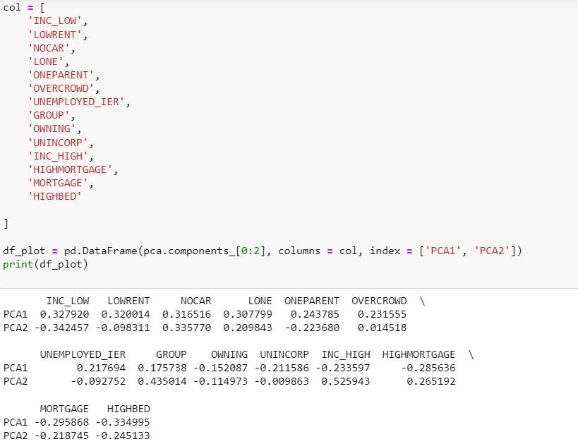
Every PC is a linear mixture of all standardized options and is differentiated solely by its respective loading of standardized options. For instance, the determine beneath reveals the load assigned by operate to the primary and his second PC (PC1 and PC2).
Utilizing 14 PCs, the code beneath visualizes how a lot variation every PC explains.
## Create visualization for variations defined by every PC

exp_var_pca = pca.explained_variance_ratio_
plt.bar(vary(1, len(exp_var_pca) + 1), exp_var_pca, alpha = 0.7,
            label = '% of Variation Defined',shade = 'darkseagreen')

plt.ylabel('Defined Variation')
plt.xlabel('Principal Element')
plt.legend(loc = 'greatest')
plt.present()
As proven within the output visualization beneath, Principal Element 1 (PC1) accounts for the most important proportion of the variance within the unique dataset, and every subsequent PC explains much less variance. Particularly, PC1 describes his circa 2015. 35% of the variation within the information.
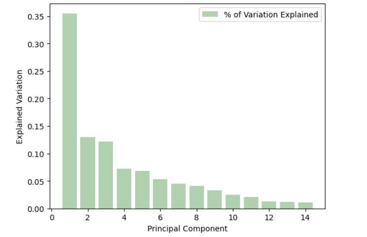
On this article’s demo, PC1 is chosen as the one PC to derive the socio-economic rating for the next causes:
- PC1 explains sufficiently massive variation within the information on a relative foundation.
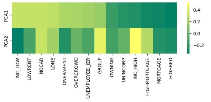
- Selecting extra PCs could clarify (barely) extra variation, however makes it tough to interpret scores that bear in mind the socio-economic benefits and downsides of particular geographic areas. For instance, as proven within the picture beneath, PC1 and PC2 present conflicting explanations of how a selected characteristic (e.g. “INC_LOW”) impacts the socio-economic variation of a geographic space. There could also be instances.
## Present and evaluate loadings for PC1 and PC2

### Utilizing df_plot dataframe per Picture 1

sns.heatmap(df_plot, annot = False, fmt = ".1f", cmap = 'summer season')
plt.present()
To acquire a rating for every SA1, merely multiply the standardized portion of every characteristic by the PC1 loading. This may be achieved by:
## Get hold of uncooked rating based mostly on PC1

### Carry out sum product of standardised characteristic and PC1 loading
pca.fit_transform(data_final)

### Reverse the signal of the sum product above to make output extra interpretable
pca_data_transformed = -1.0*pca.fit_transform(data_final)

### Convert to Pandas dataframe, and be part of uncooked rating with SA1 column
pca1 = pd.DataFrame(pca_data_transformed[:,0], columns = ['Score_Raw'])
score_SA1 = pd.concat([data1_dropna['SA1_2021'].reset_index(drop = True), pca1]
                    , axis = 1)

### Examine the uncooked rating
score_SA1.head()
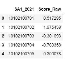
The upper the rating, the extra advantageous the SA1 is when it comes to entry to socio-economic assets.
verification
How do we all know that the rating we derived above was even remotely right?
For context, ABS truly Index of Economic Resources (IER)outlined on the ABS web site as:
“The Index of Financial Assets (IER) focuses on the monetary features of relative socio-economic benefit and drawback by summarizing variables associated to revenue and housing. variables are excluded as a result of they don’t seem to be direct measures of financial assets. We additionally exclude belongings corresponding to financial savings and shares, that are related however can’t be included as a result of they don’t seem to be collected within the census.”
With out offering detailed directions, ABS mentioned: technical paper We present that the IER was derived utilizing the identical performance (14) and methodology (PCA, PC1 solely) as carried out above. Because of this should you derive the proper scores, they need to be akin to printed IER scores. here (“Statistics Area Stage 1, Index, SEIFA 2021.xlsx”, Desk 4).
Because the printed scores are standardized to a imply of 1,000 and a normal deviation of 100, we start our validation by standardizing the uncooked scores to the identical.
## Standardise uncooked scores

score_SA1['IER_recreated'] =
          (score_SA1['Score_Raw']/score_SA1['Score_Raw'].std())*100 + 1000
For comparability, we load the IER scores printed by SA1.
## Learn in ABS printed IER scores
## equally to how we learn within the standardised portion of the options

file2 = 'information/Statistical Space Stage 1, Indexes, SEIFA 2021.xlsx'

data2 = pd.read_excel(file2, sheet_name = 'Desk 4', header = 5,
                      usecols = 'A:C')

data2.rename(columns =  {'2021 Statistical Space Stage 1 (SA1)': 'SA1_2021', 'Rating': 'IER_2021'}, inplace = True)

col_select = ['SA1_2021', 'IER_2021']
data2 = data2[col_select]

ABS_IER_dropna = data2.dropna().reset_index(drop = True)
Verification 1 — PC1 load
As proven within the determine beneath, the load of PC1 derived above is PC1 loading published by ABS means that their distinction is a continuing -45%. That is only a scaling distinction, so it doesn’t have an effect on the standardized (imply 1,000, commonplace deviation 100) derived scores.
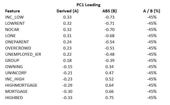
(You need to be capable to see the “Derived (A)” column within the PC1 load in picture 1).
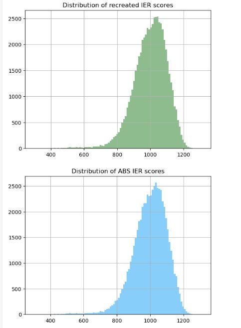
Check 2 — Distribution of scores
The code beneath creates a histogram of each scores. Their shapes look nearly an identical.
## Examine distribution of scores

score_SA1.hist(column = 'IER_recreated', bins = 100, shade = 'darkseagreen')
plt.title('Distribution of recreated IER scores')

ABS_IER_dropna.hist(column = 'IER_2021', bins = 100, shade = 'lightskyblue')
plt.title('Distribution of ABS IER scores')

plt.present()
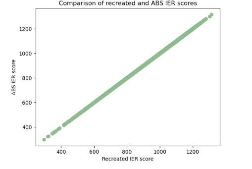
Validation 3 – IER rating with SA1
As the final word take a look at, let’s evaluate the IER scores from SA1.
## Be a part of the 2 scores by SA1 for comparability
IER_join = pd.merge(ABS_IER_dropna, score_SA1, how = 'left', on = 'SA1_2021')

## Plot scores on x-y axis.
## If scores are an identical, it ought to present a straight line.

plt.scatter('IER_recreated', 'IER_2021', information = IER_join, shade = 'darkseagreen')
plt.title('Comparability of recreated and ABS IER scores')
plt.xlabel('Recreated IER rating')
plt.ylabel('ABS IER rating')

plt.present()
A diagonal straight line, as proven within the output picture beneath, signifies that the 2 scores are almost an identical.
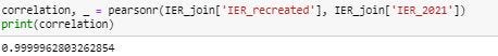
Along with this, the code beneath reveals that the 2 scores have a correlation near 1.
Ideas as a conclusion
The demonstration on this article successfully reproduces how one can modify the IER, one of many 4 socio-economic indicators printed by the ABS. The IER can be utilized to rank the socio-economic standing of a geographic space.
When you step again and give it some thought, what we have basically achieved is to scale back the dimensionality of the info from 14 to 1, and lose a number of the data that the info conveys.
Dimensionality discount strategies corresponding to PCA additionally generally assist cut back high-dimensional areas, corresponding to textual content embeddings, to 2 or three (visualizable) principal elements.
reference
[1] Australian Bureau of Statistics (2021), Regional Socio-Economic Index (SEIFA)ABS web site, accessed December 29, 2023 (creative common license)
Driving the AI/ML wave, I take pleasure in creating and sharing step-by-step guides and how-to tutorials in a complete language with ready-to-run code. If you’d like entry to all my articles (and people of different practitioners/writers on Medium), you’ll be able to join right here: Link right here!
Deriving a Rating to Present Relative Socio-Financial Benefit and Drawback of a Geographic Space initially appeared on In direction of Knowledge Science on Medium, the place individuals proceed the dialog by highlighting and responding to this story.
