A Complete Overview of Gaussian Splatting

549

All the pieces you might want to know concerning the new pattern within the discipline of 3D representations

Gaussian splatting is a technique for representing 3D scenes and rendering novel views launched in “3D Gaussian Splatting for Actual-Time Radiance Discipline Rendering”¹. It may be regarded as an alternative choice to NeRF²-like fashions, and identical to NeRF again within the day, Gaussian splatting led to lots of new research works that selected to make use of it as an underlying illustration of a 3D world for varied use instances. So what’s so particular about it and why is it higher than NeRF? Or is it, even? Let’s discover out!

Desk of contents:

• TL;DR
• Representing a 3D world
• Image formation model & rendering
• Optimization
• View-dependant colors with SH
• Limitations
• Where to play with it

TL;DR

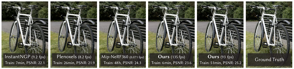
Firstly, the primary declare to fame of this work was the excessive rendering pace as could be understood from the title. That is as a result of illustration itself which can be coated under and due to the tailor-made implementation of a rendering algorithm with customized CUDA kernels.

Moreover, Gaussian splatting doesn’t contain any impartial community in any respect. There isn’t even a small MLP, nothing “neural”, a scene is actually only a set of factors in house. This in itself is already an consideration grabber. It’s fairly refreshing to see such a way gaining reputation in our AI-obsessed world with analysis corporations chasing fashions comprised of an increasing number of billions of parameters. Its thought stems from “Floor splatting”³ (2001) so it units a cool instance that basic pc imaginative and prescient approaches can nonetheless encourage related options. Its easy and specific illustration makes Gaussian splatting significantly interpretable, an excellent purpose to decide on it over NeRFs for some purposes.

Representing a 3D world

As talked about earlier, in Gaussian splatting a 3D world is represented with a set of 3D factors, in actual fact, thousands and thousands of them, in a ballpark of 0.5–5 million. Every level is a 3D Gaussian with its personal distinctive parameters which are fitted per scene such that renders of this scene match intently to the recognized dataset photos. The optimization and rendering processes can be mentioned later so let’s focus for a second on the required parameters.

Every 3D Gaussian is parametrized by:

• Imply μ interpretable as location x, y, z;
• Covariance Σ;
• Opacity σ(𝛼), a sigmoid operate is utilized to map the parameter to the [0, 1] interval;
• Colour parameters, both 3 values for (R, G, B) or spherical harmonics (SH) coefficients.

Two teams of parameters right here want additional dialogue, a covariance matrix and SH. There’s a separate part devoted to the latter. As for the covariance, it’s chosen to be anisotropic by design, that’s, not isotropic. Virtually, it signifies that a 3D level could be an ellipsoid rotated and stretched alongside any route in house. It may have required 9 parameters, nonetheless, they can’t be optimized instantly as a result of a covariance matrix has a bodily that means provided that it’s a positive semi-definite matrix. Utilizing gradient descent for optimization makes it arduous to pose such constraints on a matrix instantly, that’s the reason it’s factorized as an alternative as follows:

Such factorization is called eigendecomposition of a covariance matrix and could be understood as a configuration of an ellipsoid the place:

• S is a diagonal scaling matrix with 3 parameters for scale;
• R is a 3×3 rotation matrix analytically expressed with 4 quaternions.

The fantastic thing about utilizing Gaussians lies within the two-fold influence of every level. On one hand, every level successfully represents a restricted space in house near its imply, in accordance with its covariance. Then again, it has a theoretically infinite extent that means that every Gaussian is outlined on the entire 3D house and could be evaluated for any level. That is nice as a result of throughout optimization it permits gradients to stream from lengthy distances.⁴

The influence of a 3D Gaussian i on an arbitrary 3D level p in 3D is outlined as follows:

This equation appears to be like virtually like a chance density operate of the multivariate normal distribution besides the normalization time period with a determinant of covariance is ignored and it’s weighting by the opacity as an alternative.

Picture formation mannequin & rendering

Picture formation mannequin

Given a set of 3D factors, probably, probably the most attention-grabbing half is to see how can or not it’s used for rendering. You may be beforehand conversant in a point-wise 𝛼-blending utilized in NeRF. Seems that NeRFs and Gaussian splatting share the identical picture formation mannequin. To see this, let’s take just a little detour and re-visit the volumetric rendering components given in NeRF² and lots of of its follow-up works (1). We may even rewrite it utilizing easy transitions (2):

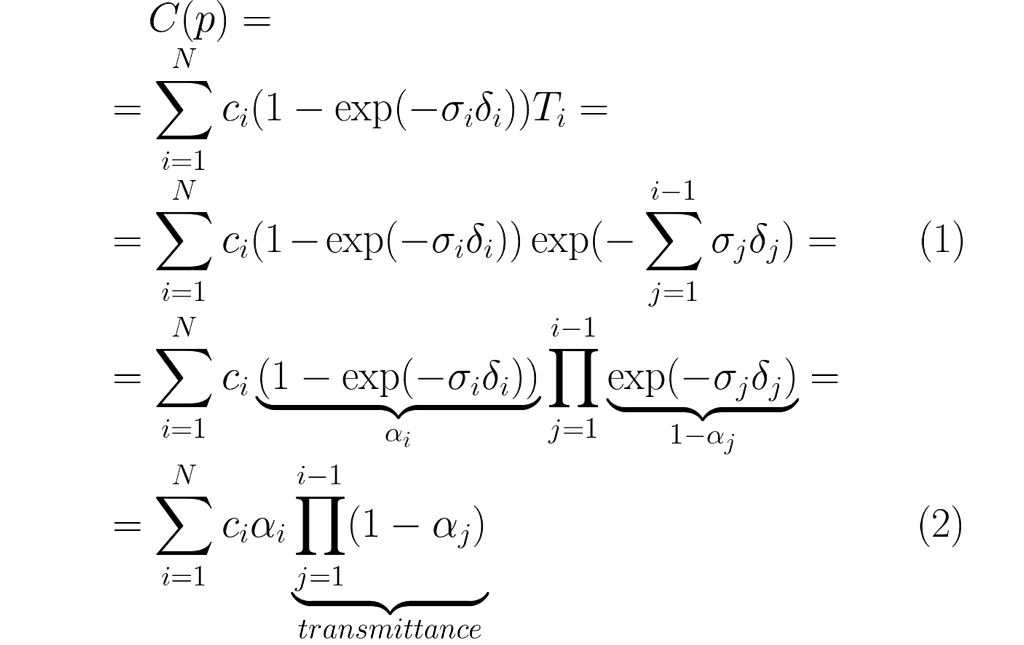
You may discuss with the NeRF paper for the definitions of σ and δ however conceptually this may be learn as follows: shade in a picture pixel p is approximated by integrating over samples alongside the ray going by means of this pixel. The ultimate shade is a weighted sum of colours of 3D factors sampled alongside this ray, down-weighted by transmittance. With this in thoughts, let’s lastly have a look at the picture formation mannequin of Gaussian splatting:

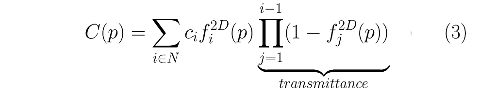
Certainly, formulation (2) and (3) are virtually similar. The one distinction is how 𝛼 is computed between the 2. Nevertheless, this small discrepancy seems extraordinarily important in follow and leads to drastically completely different rendering speeds. In actual fact, it’s the muse of the real-time efficiency of Gaussian splatting.

To know why that is the case, we have to perceive what f^{2D} means and which computational calls for it poses. This operate is just a projection of f(p) we noticed within the earlier part into 2D, i.e. onto a picture airplane of the digicam that’s being rendered. Each a 3D level and its projection are multivariate Gaussians so the influence of a projected 2D Gaussian on a pixel could be computed utilizing the identical components because the influence of a 3D Gaussian on different factors in 3D (see Determine 3). The one distinction is that the imply μ and covariance Σ should be projected into 2D which is finished utilizing derivations from EWA splatting⁵.

Means in 2D could be trivially obtained by projecting a vector μ in homogeneous coordinates (with additional 1 coordinate) into a picture airplane utilizing an intrinsic digicam matrix Okay and an extrinsic digicam matrix W=[R|t]:

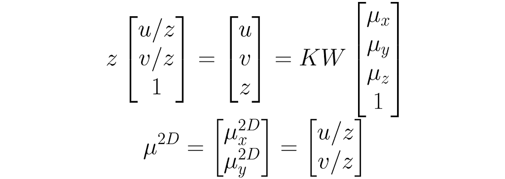
This may be additionally written in a single line as follows:

Right here “z” subscript stands for z-normalization. Covariance in 2D is outlined utilizing a Jacobian of (4), J:

The entire course of stays differentiatable, and that’s after all essential for optimization.

Rendering

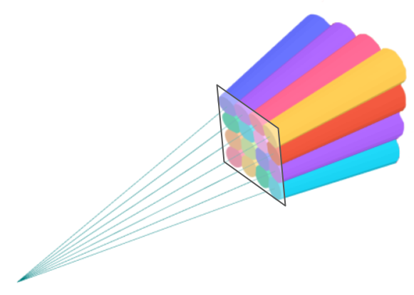
The components (3) tells us how one can get a shade in a single pixel. To render a whole picture, it’s nonetheless essential to traverse by means of all of the HxW rays, identical to in NeRF, nonetheless, the method is way more light-weight as a result of:

• For a given digicam, f(p) of every 3D level could be projected into 2D prematurely, earlier than iterating over pixels. This manner, when a Gaussian is mixed for just a few close by pixels, we received’t must re-project it again and again once more.
• There’s no MLP to be inferenced H·W·P occasions for a single picture, 2D Gaussians are blended onto a picture instantly.
• There’s no ambiguity wherein 3D level to judge alongside the ray, no want to decide on a ray sampling strategy. A set of 3D factors overlapping the ray of every pixel (see N in (3)) is discrete and glued after optimization.
• A pre-processing sorting stage is finished as soon as per body, on a GPU, utilizing a customized implementation of differentiable CUDA kernels.

The conceptual distinction could be seen in Determine 4:

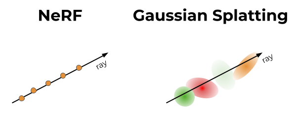
The sorting algorithm talked about above is likely one of the contributions of the paper. Its function is to arrange for shade rendering with the components (3): sorting of the 3D factors by depth (proximity to a picture airplane) and grouping them by tiles. The primary is required to compute transmittance, and the latter permits to restrict the weighted sum for every pixel to α-blending of the related 3D factors solely (or their 2D projections, to be extra particular). The grouping is achieved utilizing easy 16×16 pixel tiles and is carried out such {that a} Gaussian can land in just a few tiles if it overlaps greater than a single view frustum. Due to sorting, the rendering of every pixel could be lowered to α-blending of pre-ordered factors from the tile the pixel belongs to.

Optimization

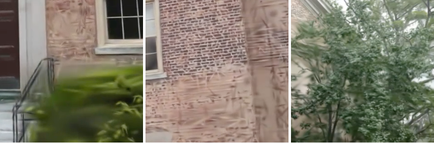
A naive query may come to thoughts: how is it even doable to get a decent-looking picture from a bunch of blobs in house? And nicely, it’s true that if Gaussians aren’t optimized correctly, you’ll get all types of pointy artifacts in renders. In Determine 6 you may observe an instance of such artifacts, they appear fairly actually like ellipsoids. The important thing to getting good renders is 3 elements: good initialization, differentiable optimization, and adaptive densification.

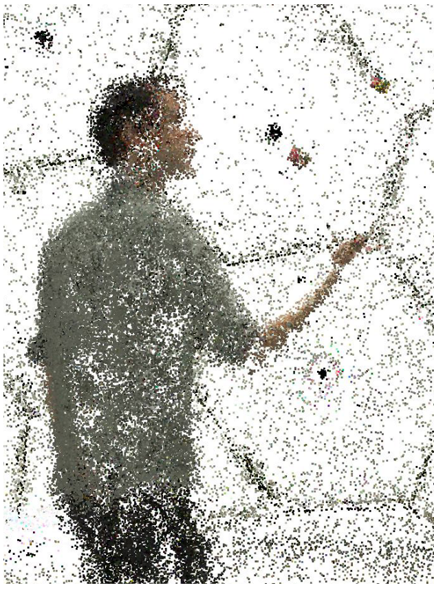
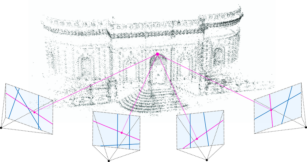
The initialization refers back to the parameters of 3D factors set at the beginning of coaching. For level places (means), the authors suggest to make use of a degree cloud produced by SfM (Construction from Movement), see Determine 7. The logic is that for any 3D reconstruction, be it with GS, NeRF, or one thing extra basic, you should know digicam matrices so you’d most likely run SfM anyway to acquire these. Since SfM produces a sparse level cloud as a by-product, why not use it for initialization? In order that’s what the paper suggests. When a degree cloud will not be out there for no matter purpose, a random initialization can be utilized as an alternative, below the chance of a possible lack of the ultimate reconstruction high quality.

Covariances are initialized to be isotropic, in different phrases, 3D factors start as spheres. The radiuses are set primarily based on imply distances to neighboring factors such that the 3D world is properly coated and has no “holes”.

After init, a easy Stochastic Gradient Descent is used to suit every little thing correctly. The scene is optimized for a loss operate that could be a mixture of L1 and D-SSIM (structural dissimilarity index measure) between a floor fact view and a present render.

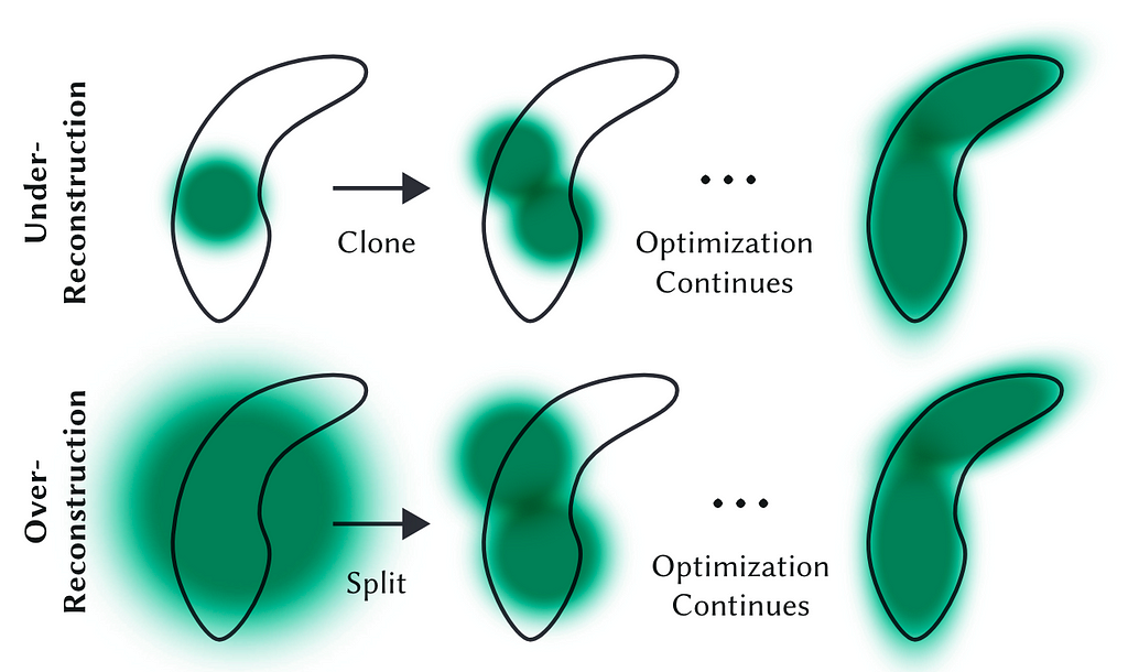
Nevertheless, that’s not it, one other essential half stays and that’s adaptive densification. It’s launched occasionally throughout coaching, say, each 100 SGD steps and its function is to deal with under- and over-reconstruction. It’s necessary to emphasise that SGD by itself can solely do as a lot as regulate the present factors. However it will wrestle to search out good parameters in areas that lack factors altogether or have too a lot of them. That’s the place adaptive densification is available in, splitting factors with massive gradients (Determine 8) and eradicating factors which have converged to very low values of α (if a degree is that clear, why hold it?).

View-dependant colours with SH

Spherical harmonics, SH for brief, play a big function in pc graphics and have been first proposed as a technique to study a view-dependant shade of discrete 3D voxels in Plenoxels⁶. View dependence is a nice-to-have property that improves the standard of renders because it permits the mannequin to characterize non-Lambertian results, e.g. specularities of metallic surfaces. Nevertheless, it’s actually not a should because it’s doable to make a simplification, select to characterize shade with 3 RGB values, and nonetheless use Gaussian splatting prefer it was executed in [4]. That’s the reason we’re reviewing this illustration element individually after the entire technique is laid out.

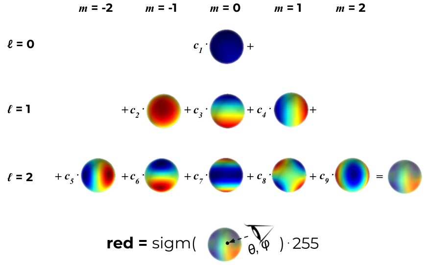
SH are particular features outlined on the floor of a sphere. In different phrases, you may consider such a operate for any level on the sphere and get a worth. All of those features are derived from this single components by selecting constructive integers for ℓ and −ℓ ≤ m ≤ ℓ, one (ℓ, m) pair per SH:

Whereas a bit intimidating at first, for small values of l this components simplifies considerably. In actual fact, for ℓ = 1, Y = ~0.282, only a fixed on the entire sphere. Quite the opposite, larger values of ℓ produce extra advanced surfaces. The speculation tells us that spherical harmonics kind an orthonormal foundation so every operate outlined on a sphere could be expressed by means of SH.

That’s why the concept to specific view-dependant shade goes like this: let’s restrict ourselves to a sure diploma of freedom ℓ_max and say that every shade (purple, inexperienced, and blue) is a linear mixture of the primary ℓ_max SH features. For each 3D Gaussian, we wish to study the right coefficients in order that once we have a look at this 3D level from a sure route it’ll convey a shade the closest to the bottom fact one. The entire means of acquiring a view-dependant shade could be seen in Determine 9.

Limitations

Regardless of the general nice outcomes and the spectacular rendering pace, the simplicity of the illustration comes with a value. Essentially the most important consideration is varied regularization heuristics which are launched throughout optimization to protect the mannequin towards “damaged” Gaussians: factors which are too massive, too lengthy, redundant, and many others. This half is essential and the talked about points could be additional amplified in duties past novel view rendering.

The selection to step apart from a steady illustration in favor of a discrete one signifies that the inductive bias of MLPs is misplaced. In NeRFs, an MLP performs an implicit interpolation and smoothes out doable inconsistencies between given views, whereas 3D Gaussians are extra delicate, main again to the issue described above.

Moreover, Gaussian splatting will not be free from some well-known artifacts current in NeRFs which they each inherit from the shared picture formation mannequin: decrease high quality in much less seen or unseen areas, floaters near a picture airplane, and many others.

The file dimension of a checkpoint is one other property to consider, although novel view rendering is way from being deployed to edge gadgets. Contemplating the ballpark variety of 3D factors and the MLP architectures of widespread NeRFs, each take the identical order of magnitude of disk house, with GS being only a few occasions heavier on common.

The place to play with it

No weblog put up can do justice to a way in addition to simply working it and seeing the outcomes for your self. Right here is the place you may play round:

• gaussian-splatting — the official implementation with customized CUDA kernels;
• nerfstudio —sure, Gaussian splatting in nerfstudio. This can be a framework initially devoted to NeRF-like fashions however since December, ‘23, it additionally helps GS;
• threestudio-3dgs — an extension for threestudio, one other cross-model framework. It’s best to use this one if you’re serious about producing 3D fashions from a immediate quite than studying an present set of photos;
• UnityGaussianSplatting — if Unity is your factor, you may port a educated mannequin into this plugin for visualization;
• gsplat — a library for CUDA-accelerated rasterization of Gaussians that branched out of nerfstudio. It may be used for impartial torch-based initiatives as a differentiatable module for splatting.

Have enjoyable!

Acknowledgments

This weblog put up relies on a gaggle assembly within the lab of Dr. Tali Dekel. Particular thanks go to Michal Geyer for the discussions of the paper and to the authors of [4] for a coherent abstract of Gaussian splatting.

References

1. Kerbl, B., Kopanas, G., Leimkühler, T., & Drettakis, G. (2023). 3D Gaussian Splatting for Real-Time Radiance Field Rendering. SIGGRAPH 2023.
2. Mildenhall, B., Srinivasan, P. P., Tancik, M., Barron, J. T., Ramamoorthi, R., & Ng, R. (2020). NeRF: Representing Scenes as Neural Radiance Fields for View Synthesis. ECCV 2020.
3. Zwicker, M., Pfister, H., van Baar, J., & Gross, M. (2001). Surface Splatting. SIGGRAPH 2001
4. Luiten, J., Kopanas, G., Leibe, B., & Ramanan, D. (2023). Dynamic 3D Gaussians: Tracking by Persistent Dynamic View Synthesis. Worldwide Convention on 3D Imaginative and prescient.
5. Zwicker, M., Pfister, H., van Baar, J., & Gross, M. (2001). EWA Volume Splatting. IEEE Visualization 2001.
6. Yu, A., Fridovich-Keil, S., Tancik, M., Chen, Q., Recht, B., & Kanazawa, A. (2023). Plenoxels: Radiance Fields without Neural Networks. CVPR 2022.

---

A Complete Overview of Gaussian Splatting was initially printed in In the direction of Knowledge Science on Medium, the place persons are persevering with the dialog by highlighting and responding to this story.