Prototyping of gradient descent in machine studying

be taught

Monitored studying is a class of machine studying that makes use of labeled datasets to coach algorithms to foretell outcomes and acknowledge patterns.

In contrast to unsupervised studying, monitored studying algorithms are given labeled coaching to be taught the connection between enter and output.

Stipulations: Linear algebra

---

I suppose now we have Regression downside The mannequin should predict steady values ​​by acquiring the variety of enter capabilities (xi).

The expected worth is outlined as a operate known as speculation (h):

the place:

• θi: the ith parameter corresponding to every enter operate (x_i)
• ϵ (Epsilon): Gaussian error (ϵ~n(0,σ²)))

---

As a result of the speculation of a single enter produces a scalar worth (hθ(x)∈R), Transposition of parameter vector (θt) and Purposeful vector of that enter (x):

Batch gradient descent

Descending slope Iterative optimization algorithm used to search out the native minimal of a operate. At every step, transfer in the wrong way from the steepest descent to regularly decrease the operate’s worth.

Now, do not forget that there are n parameters that have an effect on predictions. Subsequently, you have to know the particular contribution of Particular person parameters (θi) Helps coaching information (xi))) For capabilities.

Suppose you set the dimensions of every step as the training fee (Alpha), and the price curve (j), and the parameters are subtracted within the subsequent step, and also you get:

(Alpha: Studying fee, J (θ):cOST operate, ∂/∂θi: Partial by-product of the above price operate θi))

gradient

The gradient represents the gradient of the price operate.

Contemplating the remaining parameters and the corresponding partial by-product of the price operate (j), the gradient of the price operate at θ for the n parameter is outlined as follows:

A gradient is the matrix illustration of the partial derivatives of the price operate for all parameters (θ0 to θn).

As a result of the training fee is a scalar (α∈R), the replace guidelines for the gradient descent algorithm are expressed in matrix notation.

the consequence, The parameter (θ) resides in (n+1) dimension area.

Geographically, will probably be downhill with steps similar to studying charges till convergence is reached.

Calculation

The aim of linear regression is to reduce the hole (MSE) between the anticipated worth and the precise worth given within the coaching information set.

Value operate (goal operate)

This hole (MSE) is outlined as the common hole for all coaching examples.

the place

• jθ: Value operate (or loss operate),
• hθ: Prediction from the mannequin,
• X: i_th enter operate,
• y: i_th goal worth, and
• M: Variety of coaching examples.

gradient Calculated by the dose Partial by-product of the price operate for every parameter:

As a result of now we have n+1 parameter Format the gradient vector utilizing matrix notation (together with the intercept time period θ0) and examples of M coaching.

In a matrix notation the place x represents a design matrix containing intercept phrases and θ is a parameter vector, the gradient ∇θj(θ) is given as follows:

LMS (Least Imply Squares) Rule is an iterative algorithm that constantly adjusts the parameters of the mannequin based mostly on errors between prediction and precise goal values ​​within the coaching instance.

Least Squares (LMS) Guidelines

For every epoch Of the gradient descent, all parameters θi are up to date by subtracting a few of the imply error in all coaching examples.

This course of permits the algorithm to be discovered repeatedly Optimum parameters This minimizes the price operate.

(Observe: θi is a parameter related to enter operate XI, and the objective of the algorithm is to search out the optimum worth, not already the optimum parameter.)

Regular equation

Discover Optimum parameters (θ*) This minimizes price capabilities and is usable Regular equation.

This technique offers an analytical resolution for linear regression, permitting direct calculation of θ values ​​that decrease the price operate.

In contrast to iterative optimization methods, strange equations discover this optimum by immediately fixing factors with zero gradients, making certain instant convergence.

due to this fact:

This is dependent upon the belief of the design matrix x could be inverted,Which means all of its enter capabilities (x_0 to x_n) are Linearly unbiased.

If X isn’t invertible, the enter capabilities have to be adjusted to make sure mutual independence.

simulation

In actuality, the method is repeated till it’s set and converged.

• Value Perform and its Gradation
• Studying fee
• Resistance (minimal price threshold to cease iteration)
• Most variety of iterations
• Start line

Batch based mostly on studying fee

The next coding snippet reveals the method of gradient descent, so we discover the native minimal of the quadratic price operate with studying charges (0.1, 0.3, 0.8, 0.9).

def cost_func(x):
    return x**2 - 4 * x + 1

def gradient(x):
    return 2*x - 4

def gradient_descent(gradient, begin, learn_rate, max_iter, tol):
    x = begin
    steps = [start] # information studying steps

    for _ in vary(max_iter):
        diff = learn_rate * gradient(x)
        if np.abs(diff) < tol:
            break
        x = x - diff
        steps.append(x)

    return x, steps

x_values = np.linspace(-4, 11, 400)
y_values = cost_func(x_values)
initial_x = 9
iterations = 100
tolerance = 1e-6
learning_rates = [0.1, 0.3, 0.8, 0.9]

def gradient_descent_curve(ax, learning_rate):
    final_x, historical past = gradient_descent(gradient, initial_x, learning_rate, iterations, tolerance)

    ax.plot(x_values, y_values, label=f'Value operate: $J(x) = x^2 - 4x + 1$', lw=1, coloration='black')

    ax.scatter(historical past, [cost_func(x) for x in history], coloration='pink', zorder=5, label='Steps')
    ax.plot(historical past, [cost_func(x) for x in history], 'r--', lw=1, zorder=5)

    ax.annotate('Begin', xy=(historical past[0], cost_func(historical past[0])), xytext=(historical past[0], cost_func(historical past[0]) + 10),
                arrowprops=dict(facecolor='black', shrink=0.05), ha='middle')
    ax.annotate('Finish', xy=(final_x, cost_func(final_x)), xytext=(final_x, cost_func(final_x) + 10),
                arrowprops=dict(facecolor='black', shrink=0.05), ha='middle')
    
    ax.set_title(f'Studying Charge: {learning_rate}')
    ax.set_xlabel('Enter function: x')
    ax.set_ylabel('Value: J')
    ax.grid(True, alpha=0.5, ls='--', coloration='gray')
    ax.legend()

fig, axs = plt.subplots(1, 4, figsize=(30, 5))
fig.suptitle('Gradient Descent Steps by Studying Charge')

for ax, lr in zip(axs.flatten(), learning_rates):
    gradient_descent_curve(ax=ax, learning_rate=lr)

---

Bank card transaction prediction

Let’s use it Sample data set In Kaggle, predict bank card transactions utilizing linear regression utilizing batch GD.

1. Information Preprocessing

a) Base Information Body

First, merge these 4 information from the pattern dataset utilizing ID as key whereas sanitizing the RAW information.

• Transactions (CSV)
• Consumer (CSV)
• Credit score Card (CSV)
• train_fraud_labels(json)

# load transaction information
trx_df = pd.read_csv(f'{dir}/transactions_data.csv')

# sanitize the dataset 
trx_df = trx_df[trx_df['errors'].isna()]
trx_df = trx_df.drop(columns=['merchant_city','merchant_state', 'date', 'mcc', 'errors'], axis='columns')
trx_df['amount'] = trx_df['amount'].apply(sanitize_df)

# merge the dataframe with fraud transaction flag.
with open(f'{dir}/train_fraud_labels.json', 'r') as fp:
    fraud_labels_json = json.load(fp=fp)

fraud_labels_dict = fraud_labels_json.get('goal', {})
fraud_labels_series = pd.Sequence(fraud_labels_dict, title='is_fraud')
fraud_labels_series.index = fraud_labels_series.index.astype(int)

merged_df = pd.merge(trx_df, fraud_labels_series, left_on='id', right_index=True, how='left')
merged_df.fillna({'is_fraud': 'No'}, inplace=True)
merged_df['is_fraud'] = merged_df['is_fraud'].map({'Sure': 1, 'No': 0})
merged_df = merged_df.dropna()

# load card information
card_df = pd.read_csv(f'{dir}/cards_data.csv')
card_df = card_df.change('nan', np.nan).dropna()
card_df = card_df[card_df['card_on_dark_web'] == 'No']
card_df = card_df.drop(columns=['acct_open_date', 'card_number', 'expires', 'cvv', 'card_on_dark_web'], axis='columns')
card_df['credit_limit'] = card_df['credit_limit'].apply(sanitize_df)

# load person information
user_df = pd.read_csv(f'{dir}/users_data.csv')
user_df = user_df.drop(columns=['birth_year', 'birth_month', 'address', 'latitude', 'longitude'], axis='columns')
user_df = user_df.change('nan', np.nan).dropna()
user_df['per_capita_income'] = user_df['per_capita_income'].apply(sanitize_df)
user_df['yearly_income'] = user_df['yearly_income'].apply(sanitize_df)
user_df['total_debt'] = user_df['total_debt'].apply(sanitize_df)

# merge transaction and card information
merged_df = pd.merge(left=merged_df, proper=card_df, left_on='card_id', right_on='id', how='inside')
merged_df = pd.merge(left=merged_df, proper=user_df, left_on='client_id_x', right_on='id', how='inside')
merged_df = merged_df.drop(columns=['id_x', 'client_id_x', 'card_id', 'merchant_id', 'id_y', 'client_id_y', 'id'], axis='columns')
merged_df = merged_df.dropna()

# finalize the dataframe
categorical_cols = merged_df.select_dtypes(embody=['object']).columns
df = merged_df.copy()
df = pd.get_dummies(df, columns=categorical_cols, dummy_na=False, dtype=float)
df = df.dropna()
print('Base information body: n', df.head(n=3))

b) Preprocessing
From the bottom information body, choose the suitable enter operate, reminiscent of:
A seemingly linear relationship with steady values ​​and transaction quantities.

df = df[df['is_fraud'] == 0]
df = df[['amount', 'per_capita_income', 'yearly_income', 'credit_limit', 'credit_score', 'current_age']]

Then filter past outliers Commonplace deviations away from the three imply:

def filter_outliers(df, column, std_threshold) -> pd.DataFrame:
    imply = df[column].imply()
    std = df[column].std()
    upper_bound = imply + std_threshold * std
    lower_bound = imply - std_threshold * std
    filtered_df = df[(df[column] <= upper_bound) | (df[column] >= lower_bound)]
    return filtered_df

df = df.change(to_replace='NaN', worth=0)
df = filter_outliers(df=df, column='quantity', std_threshold=3)
df = filter_outliers(df=df, column='per_capita_income', std_threshold=3)
df = filter_outliers(df=df, column='credit_limit', std_threshold=3)

Lastly, take the logarithm of the goal worth quantity To alleviate skewed distribution:

df['amount'] = df['amount'] + 1
df['amount_log'] = np.log(df['amount'])
df = df.drop(columns=['amount'], axis='columns')
df = df.dropna()

Added to * quantity To keep away from damaging infinity lument_log column.

Last Information Body:

c) Transformer
Now you’ll be able to cut up and convert the ultimate dataframe into practice/check datasets.

categorical_features = X.select_dtypes(embody=['object']).columns.tolist()
categorical_transformer = Pipeline(steps=[('imputer', SimpleImputer(strategy='most_frequent')),('onehot', OneHotEncoder(handle_unknown='ignore'))])

numerical_features = X.select_dtypes(embody=['int64', 'float64']).columns.tolist()
numerical_transformer = Pipeline(steps=[('imputer', SimpleImputer(strategy='mean')), ('scaler', StandardScaler())])

preprocessor = ColumnTransformer(
    transformers=[
        ('num', numerical_transformer, numerical_features),
        ('cat', categorical_transformer, categorical_features)
    ]
)


X_train_processed = preprocessor.fit_transform(X_train)
X_test_processed = preprocessor.rework(X_test)

2. Outline batch GD regression

class BatchGradientDescentLinearRegressor:
    def __init__(self, learning_rate=0.01, n_iterations=1000, l2_penalty=0.01, tol=1e-4, persistence=10):
        self.learning_rate = learning_rate
        self.n_iterations = n_iterations
        self.l2_penalty = l2_penalty
        self.tol = tol
        self.persistence = persistence
        self.weights = None
        self.bias = None
        self.historical past = {'loss': [], 'grad_norm': [], 'weight':[], 'bias': [], 'val_loss': []}
        self.best_weights = None
        self.best_bias = None
        self.best_val_loss = float('inf')
        self.epochs_no_improve = 0

    def _mse_loss(self, y_true, y_pred, weights):
        m = len(y_true)
        loss = (1 / (2 * m)) * np.sum((y_pred - y_true)**2)
        l2_term = (self.l2_penalty / (2 * m)) * np.sum(weights**2)
        return loss + l2_term

    def match(self, X_train, y_train, X_val=None, y_val=None):
        n_samples, n_features = X_train.form
        self.weights = np.zeros(n_features)
        self.bias = 0

        for i in vary(self.n_iterations):
            y_pred = np.dot(X_train, self.weights) + self.bias
        
            dw = (1 / n_samples) * np.dot(X_train.T, (y_pred - y_train)) + (self.l2_penalty / n_samples) * self.weights
            db = (1 / n_samples) * np.sum(y_pred - y_train)

            loss = self._mse_loss(y_train, y_pred, self.weights)
            gradient = np.concatenate([dw, [db]])
            grad_norm = np.linalg.norm(gradient)

            # replace historical past
            self.historical past['weight'].append(self.weights[0])
            self.historical past['loss'].append(loss)
            self.historical past['grad_norm'].append(grad_norm)
            self.historical past['bias'].append(self.bias)

            # descent
            self.weights -= self.learning_rate * dw
            self.bias -= self.learning_rate * db

            if X_val isn't None and y_val isn't None:
                val_y_pred = np.dot(X_val, self.weights) + self.bias
                val_loss = self._mse_loss(y_val, val_y_pred, self.weights)
                self.historical past['val_loss'].append(val_loss)

                if val_loss < self.best_val_loss - self.tol:
                    self.best_val_loss = val_loss
                    self.best_weights = self.weights.copy()
                    self.best_bias = self.bias
                    self.epochs_no_improve = 0
                else:
                    self.epochs_no_improve += 1
                    if self.epochs_no_improve >= self.persistence:
                        print(f"Early stopping at iteration {i+1} (validation loss didn't enhance for {self.persistence} epochs)")
                        self.weights = self.best_weights
                        self.bias = self.best_bias
                        break

            if (i + 1) % 100 == 0:
                print(f"Iteration {i+1}/{self.n_iterations}, Loss: {loss:.4f}", finish="")
                if X_val isn't None:
                    print(f", Validation Loss: {val_loss:.4f}")
                else:
                    go

    def predict(self, X_test):
        return np.dot(X_test, self.weights) + self.bias

3. Prediction and analysis

mannequin = BatchGradientDescentLinearRegressor(learning_rate=0.001, n_iterations=10000, l2_penalty=0, tol=1e-5, persistence=5)
mannequin.match(X_train_processed, y_train.values)
y_pred = mannequin.predict(X_test_processed)

output:
Of the 5 enter capabilities, per_capita_income The very best correlation with transaction quantity was proven.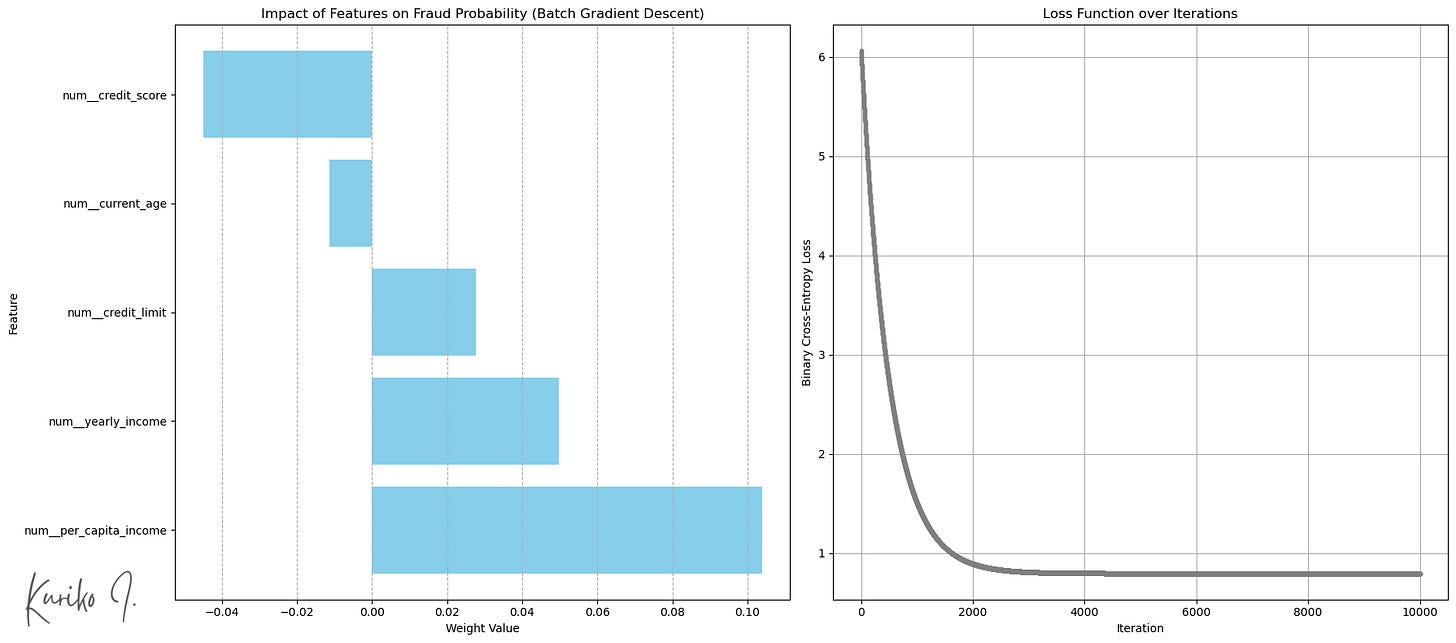

(Left: Weight by enter operate (Backside: Extra transactions), Proper: Value operate (Learning_rate = 0.001, I = 10,000, M = 50,000, n = 5))

Imply Sq. Error (MSE): 1.5752
R-squared: 0.0206
Imply Absolute Error (MAE): 1.0472

Time complexity: Coaching: o(n²m +n³) + Prediction: o(n)
House Complexity: O(nm)
(M: coaching instance dimension, n: enter operate dimension, m >>> n)

---

Stochastic gradient descent

Utilized by Batch GD All the coaching information set Computing the gradient at every iteration step (epoch) is computationally costly, particularly when you’ve gotten thousands and thousands of information units.

Stochastic gradient descent (SGD) then again,

1. Normally, coaching information is shuffled at the start of every epoch,
2. Choose it randomly a single Examples of coaching In every iteration,
3. Calculate the gradient utilizing the instance
4. Updates mannequin weights and bias After processing particular person coaching examples.

This ends in many weight updates per epoch (equal to the variety of coaching samples), many fast and computationally cheap updates based mostly on particular person information factors. It may be repeated a lot sooner by way of massive datasets.

simulation

Similar to Batch GD, it defines an SGD class and performs predictions.

class StochasticGradientDescentLinearRegressor:
    def __init__(self, learning_rate=0.01, n_iterations=100, l2_penalty=0.01, random_state=None):
        self.learning_rate = learning_rate
        self.n_iterations = n_iterations
        self.l2_penalty = l2_penalty
        self.random_state = random_state
        self._rng = np.random.default_rng(seed=random_state)
        self.weights_history = []
        self.bias_history = []
        self.loss_history = []
        self.weights = None
        self.bias = None

    def _mse_loss_single(self, y_true, y_pred):
        return 0.5 * (y_pred - y_true)**2

    def match(self, X, y):
        n_samples, n_features = X.form
        self.weights = self._rng.random(n_features)
        self.bias = 0.0

        for epoch in vary(self.n_iterations):
            permutation = self._rng.permutation(n_samples)
            X_shuffled = X[permutation]
            y_shuffled = y[permutation]

            epoch_loss = 0
            for i in vary(n_samples):
                xi = X_shuffled[i]
                yi = y_shuffled[i]

                y_pred = np.dot(xi, self.weights) + self.bias
                dw = xi * (y_pred - yi) + self.l2_penalty * self.weights
                db = y_pred - yi

                self.weights -= self.learning_rate * dw
                self.bias -= self.learning_rate * db
                epoch_loss += self._mse_loss_single(yi, y_pred)

                if n_features >= 2:
                    self.weights_history.append(self.weights[:2].copy())
                elif n_features == 1:
                    self.weights_history.append(np.array([self.weights[0], 0]))
                self.bias_history.append(self.bias)
                self.loss_history.append(self._mse_loss_single(yi, y_pred) + (self.l2_penalty / (2 * n_samples)) * (np.sum(self.weights**2) + self.bias**2)) # Approx L2

            print(f"Epoch {epoch+1}/{self.n_iterations}, Loss: {epoch_loss/n_samples:.4f}")

    def predict(self, X):
        return np.dot(X, self.weights) + self.bias

mannequin = StochasticGradientDescentLinearRegressor(learning_rate=0.001, n_iterations=200, random_state=42)
mannequin.match(X=X_train_processed, y=y_train.values)
y_pred = mannequin.predict(X_test_processed)

output:

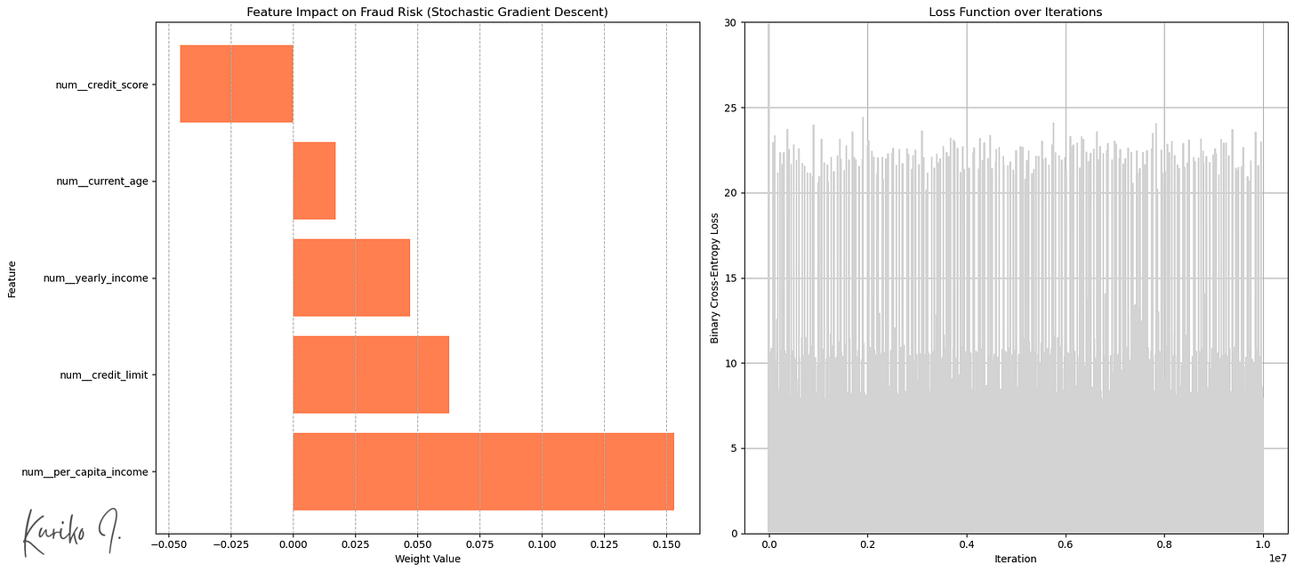
Left: Weight based mostly on enter operate, Proper: Value operate (Learning_rate= 0.001, i = 200, m = 50,000, n = 5)

SGD has been launched Randomness The optimization course of (proper of the determine).

this “noise” Can help algorithms Hopping out of shallow native minimal or saddle factors You might discover a higher space of ​​the parameter area.

consequence:
Imply Sq. Error (MSE): 1.5808
R-squared: 0.0172
Common Absolute Error (MAE): 1.0475

Time complexity: Coaching: o(n²m +n³) + Prediction: o(n)
House Complexity: o(n)
(M: coaching instance dimension, n: enter operate dimension, m >>> n)

---

Conclusion

then again Easy linear mannequin It’s computationally environment friendly, and its inherent simplicity typically prevents the seize of advanced relationships throughout the information.

Take into account commerce off Of the assorted modeling approaches to a specific goal, it’s important to reaching optimum outcomes.

---

reference

Except in any other case acknowledged, all pictures are from the writer.

This text makes use of artificial information. Licensed under Apache 2.0 for commercial use.

---

Writer: Iwai Kuriko

portfolio / LinkedIn / github