


When deploying a big language mannequin (LLM), machine studying (ML) practitioners usually care about two measurements for mannequin serving efficiency: latency, outlined by the point it takes to generate a single token, and throughput, outlined by the variety of tokens generated per second. Though a single request to the deployed endpoint would exhibit a throughput roughly equal to the inverse of mannequin latency, this isn’t essentially the case when a number of concurrent requests are concurrently despatched to the endpoint. On account of mannequin serving methods, comparable to client-side steady batching of concurrent requests, latency and throughput have a posh relationship that varies considerably primarily based on mannequin structure, serving configurations, occasion kind {hardware}, variety of concurrent requests, and variations in enter payloads comparable to variety of enter tokens and output tokens.
This put up explores these relationships by way of a complete benchmarking of LLMs out there in Amazon SageMaker JumpStart, together with Llama 2, Falcon, and Mistral variants. With SageMaker JumpStart, ML practitioners can select from a broad choice of publicly out there basis fashions to deploy to devoted Amazon SageMaker situations inside a network-isolated atmosphere. We offer theoretical ideas on how accelerator specs impression LLM benchmarking. We additionally display the impression of deploying a number of situations behind a single endpoint. Lastly, we offer sensible suggestions for tailoring the SageMaker JumpStart deployment course of to align along with your necessities on latency, throughput, value, and constraints on out there occasion varieties. All of the benchmarking outcomes in addition to suggestions are primarily based on a flexible notebook you can adapt to your use case.
Deployed endpoint benchmarking
The next determine exhibits the bottom latencies (left) and highest throughput (proper) values for deployment configurations throughout a wide range of mannequin varieties and occasion varieties. Importantly, every of those mannequin deployments use default configurations as supplied by SageMaker JumpStart given the specified mannequin ID and occasion kind for deployment.
These latency and throughput values correspond to payloads with 256 enter tokens and 256 output tokens. The bottom latency configuration limits mannequin serving to a single concurrent request, and the best throughput configuration maximizes the doable variety of concurrent requests. As we will see in our benchmarking, rising concurrent requests monotonically will increase throughput with diminishing enchancment for giant concurrent requests. Moreover, fashions are totally sharded on the supported occasion. For instance, as a result of the ml.g5.48xlarge occasion has 8 GPUs, all SageMaker JumpStart fashions utilizing this occasion are sharded utilizing tensor parallelism on all eight out there accelerators.
We will be aware a number of takeaways from this determine. First, not all fashions are supported on all situations; some smaller fashions, comparable to Falcon 7B, don’t help mannequin sharding, whereas bigger fashions have larger compute useful resource necessities. Second, as sharding will increase, efficiency usually improves, however might not essentially enhance for small fashions. It’s because small fashions comparable to 7B and 13B incur a considerable communication overhead when sharded throughout too many accelerators. We talk about this in additional depth later. Lastly, ml.p4d.24xlarge situations are inclined to have considerably higher throughput resulting from reminiscence bandwidth enhancements of A100 over A10G GPUs. As we talk about later, the choice to make use of a selected occasion kind is dependent upon your deployment necessities, together with latency, throughput, and value constraints.
How will you acquire these lowest latency and highest throughput configuration values? Let’s begin by plotting latency vs. throughput for a Llama 2 7B endpoint on an ml.g5.12xlarge occasion for a payload with 256 enter tokens and 256 output tokens, as seen within the following curve. An identical curve exists for each deployed LLM endpoint.
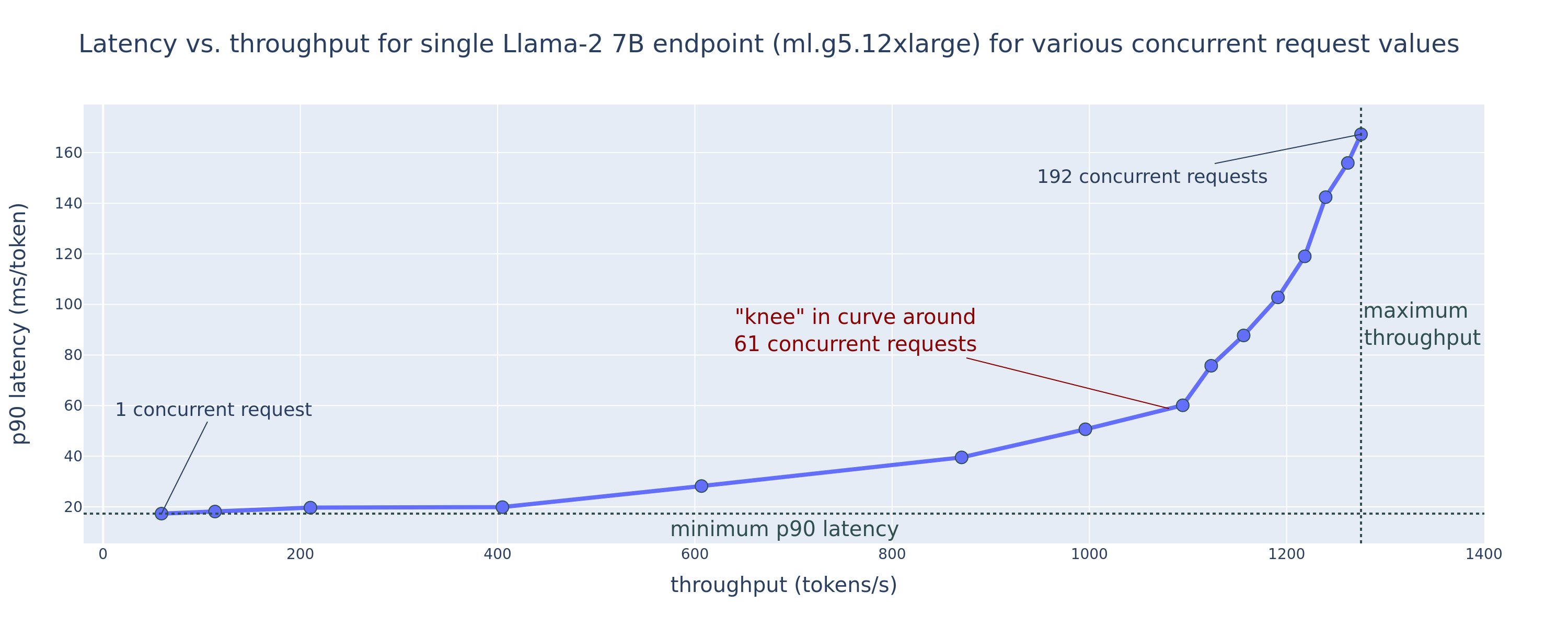
As concurrency will increase, throughput and latency additionally monotonically enhance. Subsequently, the bottom latency level happens at a concurrent request worth of 1, and you’ll cost-effectively enhance system throughput by rising concurrent requests. There exists a definite “knee” on this curve, the place it’s apparent that the throughput beneficial properties related to further concurrency don’t outweigh the related enhance in latency. The precise location of this knee is use case-specific; some practitioners might outline the knee on the level the place a pre-specified latency requirement is exceeded (for instance, 100 ms/token), whereas others might use load take a look at benchmarks and queueing idea strategies just like the half-latency rule, and others might use theoretical accelerator specs.
We additionally be aware that the utmost variety of concurrent requests is proscribed. Within the previous determine, the road hint ends with 192 concurrent requests. The supply of this limitation is the SageMaker invocation timeout restrict, the place SageMaker endpoints timeout an invocation response after 60 seconds. This setting is account-specific and never configurable for a person endpoint. For LLMs, producing a lot of output tokens can take seconds and even minutes. Subsequently, giant enter or output payloads may cause the invocation requests to fail. Moreover, if the variety of concurrent requests may be very giant, then many requests will expertise giant queue occasions, driving this 60-second timeout restrict. For the aim of this research, we use the timeout restrict to outline the utmost throughput doable for a mannequin deployment. Importantly, though a SageMaker endpoint might deal with a lot of concurrent requests with out observing an invocation response timeout, chances are you’ll need to outline most concurrent requests with respect to the knee within the latency-throughput curve. That is doubtless the purpose at which you begin to contemplate horizontal scaling, the place a single endpoint provisions a number of situations with mannequin replicas and cargo balances incoming requests between the replicas, to help extra concurrent requests.
Taking this one step additional, the next desk incorporates benchmarking outcomes for various configurations for the Llama 2 7B mannequin, together with completely different variety of enter and output tokens, occasion varieties, and variety of concurrent requests. Be aware that the previous determine solely plots a single row of this desk.
| . | Throughput (tokens/sec) | Latency (ms/token) | ||||||||||||||||||
| Concurrent Requests | 1 | 2 | 4 | 8 | 16 | 32 | 64 | 128 | 256 | 512 | 1 | 2 | 4 | 8 | 16 | 32 | 64 | 128 | 256 | 512 |
| Variety of complete tokens: 512, Variety of output tokens: 256 | ||||||||||||||||||||
| ml.g5.2xlarge | 30 | 54 | 115 | 208 | 343 | 475 | 486 | — | — | — | 33 | 33 | 35 | 39 | 48 | 97 | 159 | — | — | — |
| ml.g5.12xlarge | 59 | 117 | 223 | 406 | 616 | 866 | 1098 | 1214 | — | — | 17 | 17 | 18 | 20 | 27 | 38 | 60 | 112 | — | — |
| ml.g5.48xlarge | 56 | 108 | 202 | 366 | 522 | 660 | 707 | 804 | — | — | 18 | 18 | 19 | 22 | 32 | 50 | 101 | 171 | — | — |
| ml.p4d.24xlarge | 49 | 85 | 178 | 353 | 654 | 1079 | 1544 | 2312 | 2905 | 2944 | 21 | 23 | 22 | 23 | 26 | 31 | 44 | 58 | 92 | 165 |
| Variety of complete tokens: 4096, Variety of output tokens: 256 | ||||||||||||||||||||
| ml.g5.2xlarge | 20 | 36 | 48 | 49 | — | — | — | — | — | — | 48 | 57 | 104 | 170 | — | — | — | — | — | — |
| ml.g5.12xlarge | 33 | 58 | 90 | 123 | 142 | — | — | — | — | — | 31 | 34 | 48 | 73 | 132 | — | — | — | — | — |
| ml.g5.48xlarge | 31 | 48 | 66 | 82 | — | — | — | — | — | — | 31 | 43 | 68 | 120 | — | — | — | — | — | — |
| ml.p4d.24xlarge | 39 | 73 | 124 | 202 | 278 | 290 | — | — | — | — | 26 | 27 | 33 | 43 | 66 | 107 | — | — | — | — |
We observe some further patterns on this knowledge. When rising context dimension, latency will increase and throughput decreases. As an illustration, on ml.g5.2xlarge with a concurrency of 1, throughput is 30 tokens/sec when the variety of complete tokens is 512, vs. 20 tokens/sec if the variety of complete tokens is 4,096. It’s because it takes extra time to course of the bigger enter. We will additionally see that rising GPU functionality and sharding impacts the utmost throughput and most supported concurrent requests. The desk exhibits that Llama 2 7B has notably completely different most throughput values for various occasion varieties, and these most throughput values happen at completely different values of concurrent requests. These traits would drive an ML practitioner to justify the price of one occasion over one other. For instance, given a low latency requirement, the practitioner would possibly choose an ml.g5.12xlarge occasion (4 A10G GPUs) over an ml.g5.2xlarge occasion (1 A10G GPU). If given a excessive throughput requirement, the usage of an ml.p4d.24xlarge occasion (8 A100 GPUs) with full sharding would solely be justified underneath excessive concurrency. Be aware, nevertheless, that it’s usually helpful to as a substitute load a number of inference parts of a 7B mannequin on a single ml.p4d.24xlarge occasion; such multi-model help is mentioned later on this put up.
The previous observations had been made for the Llama 2 7B mannequin. Nonetheless, comparable patterns stay true for different fashions as properly. A main takeaway is that latency and throughput efficiency numbers are depending on payload, occasion kind, and variety of concurrent requests, so you will want to search out the best configuration to your particular utility. To generate the previous numbers to your use case, you possibly can run the linked notebook, the place you possibly can configure this load take a look at evaluation to your mannequin, occasion kind, and payload.
Making sense of accelerator specs
Deciding on appropriate {hardware} for LLM inference depends closely on particular use instances, person expertise targets, and the chosen LLM. This part makes an attempt to create an understanding of the knee within the latency-throughput curve with respect to high-level ideas primarily based on accelerator specs. These ideas alone don’t suffice to decide: actual benchmarks are mandatory. The time period gadget is used right here to embody all ML {hardware} accelerators. We assert the knee within the latency-throughput curve is pushed by one in all two elements:
- The accelerator has exhausted reminiscence to cache KV matrices, so subsequent requests are queued
- The accelerator nonetheless has spare reminiscence for the KV cache, however is utilizing a big sufficient batch dimension that processing time is pushed by compute operation latency somewhat than reminiscence bandwidth
We usually choose to be restricted by the second issue as a result of this means the accelerator sources are saturated. Principally, you’re maximizing the sources you payed for. Let’s discover this assertion in larger element.
KV caching and gadget reminiscence
Customary transformer consideration mechanisms compute consideration for every new token towards all earlier tokens. Most fashionable ML servers cache consideration keys and values in gadget reminiscence (DRAM) to keep away from re-computation at each step. That is referred to as this the KV cache, and it grows with batch dimension and sequence size. It defines what number of person requests will be served in parallel and can decide the knee within the latency-throughput curve if the compute-bound regime within the second state of affairs talked about earlier shouldn’t be but met, given the out there DRAM. The next formulation is a tough approximation for the utmost KV cache dimension.

On this formulation, B is batch dimension and N is variety of accelerators. For instance, the Llama 2 7B mannequin in FP16 (2 bytes/parameter) served on an A10G GPU (24 GB DRAM) consumes roughly 14 GB, leaving 10 GB for the KV cache. Plugging within the mannequin’s full context size (N = 4096) and remaining parameters (n_layers=32, n_kv_attention_heads=32, and d_attention_head=128), this expression exhibits we’re restricted to serving a batch dimension of 4 customers in parallel resulting from DRAM constraints. In the event you observe the corresponding benchmarks within the earlier desk, it is a good approximation for the noticed knee on this latency-throughput curve. Strategies comparable to grouped query attention (GQA) can cut back the KV cache dimension, in GQA’s case by the identical issue it reduces the variety of KV heads.
Arithmetic depth and gadget reminiscence bandwidth
The expansion within the computational energy of ML accelerators has outpaced their reminiscence bandwidth, that means they will carry out many extra computations on every byte of knowledge within the period of time it takes to entry that byte.
The arithmetic depth, or the ratio of compute operations to reminiscence accesses, for an operation determines whether it is restricted by reminiscence bandwidth or compute capability on the chosen {hardware}. For instance, an A10G GPU (g5 occasion kind household) with 70 TFLOPS FP16 and 600 GB/sec bandwidth can compute roughly 116 ops/byte. An A100 GPU (p4d occasion kind household) can compute roughly 208 ops/byte. If the arithmetic depth for a transformer mannequin is underneath that worth, it’s memory-bound; whether it is above, it’s compute-bound. The eye mechanism for Llama 2 7B requires 62 ops/byte for batch dimension 1 (for an evidence, see A guide to LLM inference and performance), which implies it’s memory-bound. When the eye mechanism is memory-bound, costly FLOPS are left unutilized.
There are two methods to higher make the most of the accelerator and enhance arithmetic depth: cut back the required reminiscence accesses for the operation (that is what FlashAttention focuses on) or enhance the batch dimension. Nonetheless, we’d not have the ability to enhance our batch dimension sufficient to achieve a compute-bound regime if our DRAM is just too small to carry the corresponding KV cache. A crude approximation of the vital batch dimension B* that separates compute-bound from memory-bound regimes for traditional GPT decoder inference is described by the next expression, the place A_mb is the accelerator reminiscence bandwidth, A_f is accelerator FLOPS, and N is the variety of accelerators. This vital batch dimension will be derived by discovering the place reminiscence entry time equals computation time. Discuss with this blog post to know Equation 2 and its assumptions in larger element.
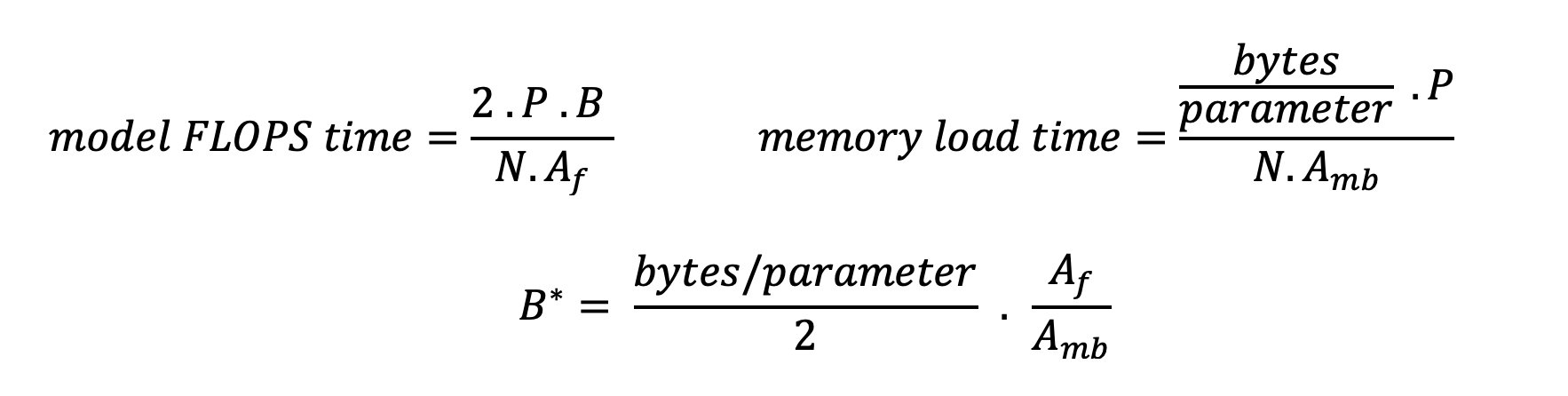
This is identical ops/byte ratio we beforehand calculated for A10G, so the vital batch dimension on this GPU is 116. One approach to strategy this theoretical, vital batch dimension is to extend mannequin sharding and cut up the cache throughout extra N accelerators. This successfully will increase the KV cache capability in addition to the memory-bound batch dimension.
One other good thing about mannequin sharding is splitting mannequin parameter and knowledge loading work throughout N accelerators. Any such sharding is a sort of mannequin parallelism additionally known as tensor parallelism. Naively, there’s N occasions the reminiscence bandwidth and compute energy in mixture. Assuming no overhead of any type (communication, software program, and so forth), this may lower decoding latency per token by N if we’re memory-bound, as a result of token decoding latency on this regime is sure by the point it takes to load the mannequin weights and cache. In actual life, nevertheless, rising the diploma of sharding leads to elevated communication between gadgets to share intermediate activations at each mannequin layer. This communication velocity is proscribed by the gadget interconnect bandwidth. It’s tough to estimate its impression exactly (for particulars, see Model parallelism), however this will finally cease yielding advantages or deteriorate efficiency — that is very true for smaller fashions, as a result of smaller knowledge transfers result in decrease switch charges.
To match ML accelerators primarily based on their specs, we advocate the next. First, calculate the approximate vital batch dimension for every accelerator kind in line with the second equation and the KV cache dimension for the vital batch dimension in line with the primary equation. You’ll be able to then use the out there DRAM on the accelerator to calculate the minimal variety of accelerators required to suit the KV cache and mannequin parameters. If deciding between a number of accelerators, prioritize accelerators so as of lowest value per GB/sec of reminiscence bandwidth. Lastly, benchmark these configurations and confirm what’s the greatest value/token to your higher sure of desired latency.
Choose an endpoint deployment configuration
Many LLMs distributed by SageMaker JumpStart use the text-generation-inference (TGI) SageMaker container for mannequin serving. The next desk discusses learn how to alter a wide range of mannequin serving parameters to both have an effect on mannequin serving which impacts the latency-throughput curve or shield the endpoint towards requests that may overload the endpoint. These are the first parameters you should use to configure your endpoint deployment to your use case. Except in any other case specified, we use default text generation payload parameters and TGI environment variables.
| Surroundings Variable | Description | SageMaker JumpStart Default Worth |
| Mannequin serving configurations | . | . |
MAX_BATCH_PREFILL_TOKENS |
Limits the variety of tokens within the prefill operation. This operation generates the KV cache for a brand new enter immediate sequence. It’s reminiscence intensive and compute sure, so this worth caps the variety of tokens allowed in a single prefill operation. Decoding steps for different queries pause whereas prefill is happening. | 4096 (TGI default) or model-specific most supported context size (SageMaker JumpStart supplied), whichever is larger. |
MAX_BATCH_TOTAL_TOKENS |
Controls the utmost variety of tokens to incorporate inside a batch throughout decoding, or a single ahead cross by the mannequin. Ideally, that is set to maximise the utilization of all out there {hardware}. | Not specified (TGI default). TGI will set this worth with respect to remaining CUDA reminiscence throughout mannequin heat up. |
SM_NUM_GPUS |
The variety of shards to make use of. That’s, the variety of GPUs used to run the mannequin utilizing tensor parallelism. | Occasion dependent (SageMaker JumpStart supplied). For every supported occasion for a given mannequin, SageMaker JumpStart supplies one of the best setting for tensor parallelism. |
| Configurations to protect your endpoint (set these to your use case) | . | . |
MAX_TOTAL_TOKENS |
This caps the reminiscence price range of a single shopper request by limiting the variety of tokens within the enter sequence plus the variety of tokens within the output sequence (the max_new_tokens payload parameter). |
Mannequin-specific most supported context size. For instance, 4096 for Llama 2. |
MAX_INPUT_LENGTH |
Identifies the utmost allowed variety of tokens within the enter sequence for a single shopper request. Issues to contemplate when rising this worth embody: longer enter sequences require extra reminiscence, which impacts steady batching, and plenty of fashions have a supported context size that shouldn’t be exceeded. | Mannequin-specific most supported context size. For instance, 4095 for Llama 2. |
MAX_CONCURRENT_REQUESTS |
The utmost variety of concurrent requests allowed by the deployed endpoint. New requests past this restrict will instantly elevate a mannequin overloaded error to forestall poor latency for the present processing requests. | 128 (TGI default). This setting means that you can acquire excessive throughput for a wide range of use instances, however it’s best to pin as acceptable to mitigate SageMaker invocation timeout errors. |
The TGI server makes use of steady batching, which dynamically batches concurrent requests collectively to share a single mannequin inference ahead cross. There are two kinds of ahead passes: prefill and decode. Every new request should run a single prefill ahead cross to populate the KV cache for the enter sequence tokens. After the KV cache is populated, a decode ahead cross performs a single next-token prediction for all batched requests, which is iteratively repeated to provide the output sequence. As new requests are despatched to the server, the subsequent decode step should wait so the prefill step can run for the brand new requests. This should happen earlier than these new requests are included in subsequent constantly batched decode steps. On account of {hardware} constraints, the continual batching used for decoding might not embody all requests. At this level, requests enter a processing queue and inference latency begins to considerably enhance with solely minor throughput achieve.
It’s doable to separate LLM latency benchmarking analyses into prefill latency, decode latency, and queue latency. The time consumed by every of those parts is basically completely different in nature: prefill is a one-time computation, decoding happens one time for every token within the output sequence, and queueing entails server batching processes. When a number of concurrent requests are being processed, it turns into tough to disentangle the latencies from every of those parts as a result of the latency skilled by any given shopper request entails queue latencies pushed by the necessity to prefill new concurrent requests in addition to queue latencies pushed by the inclusion of the request in batch decoding processes. Because of this, this put up focuses on end-to-end processing latency. The knee within the latency-throughput curve happens on the level of saturation the place queue latencies begin to considerably enhance. This phenomenon happens for any mannequin inference server and is pushed by accelerator specs.
Frequent necessities throughout deployment embody satisfying a minimal required throughput, most allowed latency, most value per hour, and most value to generate 1 million tokens. You must situation these necessities on payloads that signify end-user requests. A design to fulfill these necessities ought to contemplate many elements, together with the precise mannequin structure, dimension of the mannequin, occasion varieties, and occasion rely (horizontal scaling). Within the following sections, we concentrate on deploying endpoints to attenuate latency, maximize throughput, and reduce value. This evaluation considers 512 complete tokens and 256 output tokens.
Decrease latency
Latency is a crucial requirement in lots of real-time use instances. Within the following desk, we take a look at minimal latency for every mannequin and every occasion kind. You’ll be able to obtain minimal latency by setting MAX_CONCURRENT_REQUESTS = 1.
| Minimal Latency (ms/token) | |||||
| Mannequin ID | ml.g5.2xlarge | ml.g5.12xlarge | ml.g5.48xlarge | ml.p4d.24xlarge | ml.p4de.24xlarge |
| Llama 2 7B | 33 | 17 | 18 | 20 | — |
| Llama 2 7B Chat | 33 | 17 | 18 | 20 | — |
| Llama 2 13B | — | 22 | 23 | 23 | — |
| Llama 2 13B Chat | — | 23 | 23 | 23 | — |
| Llama 2 70B | — | — | 57 | 43 | — |
| Llama 2 70B Chat | — | — | 57 | 45 | — |
| Mistral 7B | 35 | — | — | — | — |
| Mistral 7B Instruct | 35 | — | — | — | — |
| Mixtral 8x7B | — | — | 33 | 27 | — |
| Falcon 7B | 33 | — | — | — | — |
| Falcon 7B Instruct | 33 | — | — | — | — |
| Falcon 40B | — | 53 | 33 | 27 | — |
| Falcon 40B Instruct | — | 53 | 33 | 28 | — |
| Falcon 180B | — | — | — | — | 42 |
| Falcon 180B Chat | — | — | — | — | 42 |
To attain minimal latency for a mannequin, you should use the next code whereas substituting your required mannequin ID and occasion kind:
Be aware that the latency numbers change relying on the variety of enter and output tokens. Nonetheless, the deployment course of stays the identical besides the atmosphere variables MAX_INPUT_TOKENS and MAX_TOTAL_TOKENS. Right here, these atmosphere variables are set to assist assure endpoint latency necessities as a result of bigger enter sequences might violate the latency requirement. Be aware that SageMaker JumpStart already supplies the opposite optimum atmosphere variables when deciding on occasion kind; as an illustration, utilizing ml.g5.12xlarge will set SM_NUM_GPUS to 4 within the mannequin atmosphere.
Maximize throughput
On this part, we maximize the variety of generated tokens per second. That is usually achieved on the most legitimate concurrent requests for the mannequin and the occasion kind. Within the following desk, we report the throughput achieved on the largest concurrent request worth achieved earlier than encountering a SageMaker invocation timeout for any request.
| Most Throughput (tokens/sec), Concurrent Requests | |||||
| Mannequin ID | ml.g5.2xlarge | ml.g5.12xlarge | ml.g5.48xlarge | ml.p4d.24xlarge | ml.p4de.24xlarge |
| Llama 2 7B | 486 (64) | 1214 (128) | 804 (128) | 2945 (512) | — |
| Llama 2 7B Chat | 493 (64) | 1207 (128) | 932 (128) | 3012 (512) | — |
| Llama 2 13B | — | 787 (128) | 496 (64) | 3245 (512) | — |
| Llama 2 13B Chat | — | 782 (128) | 505 (64) | 3310 (512) | — |
| Llama 2 70B | — | — | 124 (16) | 1585 (256) | — |
| Llama 2 70B Chat | — | — | 114 (16) | 1546 (256) | — |
| Mistral 7B | 947 (64) | — | — | — | — |
| Mistral 7B Instruct | 986 (128) | — | — | — | — |
| Mixtral 8x7B | — | — | 701 (128) | 3196 (512) | — |
| Falcon 7B | 1340 (128) | — | — | — | — |
| Falcon 7B Instruct | 1313 (128) | — | — | — | — |
| Falcon 40B | — | 244 (32) | 382 (64) | 2699 (512) | — |
| Falcon 40B Instruct | — | 245 (32) | 415 (64) | 2675 (512) | — |
| Falcon 180B | — | — | — | — | 1100 (128) |
| Falcon 180B Chat | — | — | — | — | 1081 (128) |
To attain most throughput for a mannequin, you should use the next code:
Be aware that the utmost variety of concurrent requests is dependent upon the mannequin kind, occasion kind, most variety of enter tokens, and most variety of output tokens. Subsequently, it’s best to set these parameters earlier than setting MAX_CONCURRENT_REQUESTS.
Additionally be aware {that a} person eager about minimizing latency is commonly at odds with a person eager about maximizing throughput. The previous is eager about real-time responses, whereas the latter is eager about batch processing such that the endpoint queue is all the time saturated, thereby minimizing processing downtime. Customers who need to maximize throughput conditioned on latency necessities are sometimes eager about working on the knee within the latency-throughput curve.
Decrease value
The primary choice to attenuate value entails minimizing value per hour. With this, you possibly can deploy a particular mannequin on the SageMaker occasion with the bottom value per hour. For real-time pricing of SageMaker situations, seek advice from Amazon SageMaker pricing. Normally, the default occasion kind for SageMaker JumpStart LLMs is the lowest-cost deployment choice.
The second choice to attenuate value entails minimizing the fee to generate 1 million tokens. This can be a easy transformation of the desk we mentioned earlier to maximise throughput, the place you possibly can first compute the time it takes in hours to generate 1 million tokens (1e6 / throughput / 3600). You’ll be able to then multiply this time to generate 1 million tokens with the value per hour of the required SageMaker occasion.
Be aware that situations with the bottom value per hour aren’t the identical as situations with the bottom value to generate 1 million tokens. As an illustration, if the invocation requests are sporadic, an occasion with the bottom value per hour could be optimum, whereas within the throttling situations, the bottom value to generate one million tokens could be extra acceptable.
Tensor parallel vs. multi-model trade-off
In all earlier analyses, we thought of deploying a single mannequin reproduction with a tensor parallel diploma equal to the variety of GPUs on the deployment occasion kind. That is the default SageMaker JumpStart habits. Nonetheless, as beforehand famous, sharding a mannequin can enhance mannequin latency and throughput solely as much as a sure restrict, past which inter-device communication necessities dominate computation time. This suggests that it’s usually helpful to deploy a number of fashions with a decrease tensor parallel diploma on a single occasion somewhat than a single mannequin with the next tensor parallel diploma.
Right here, we deploy Llama 2 7B and 13B endpoints on ml.p4d.24xlarge situations with tensor parallel (TP) levels of 1, 2, 4, and eight. For readability in mannequin habits, every of those endpoints solely load a single mannequin.
| . | Throughput (tokens/sec) | Latency (ms/token) | ||||||||||||||||||
| Concurrent Requests | 1 | 2 | 4 | 8 | 16 | 32 | 64 | 128 | 256 | 512 | 1 | 2 | 4 | 8 | 16 | 32 | 64 | 128 | 256 | 512 |
| TP Diploma | Llama 2 13B | |||||||||||||||||||
| 1 | 38 | 74 | 147 | 278 | 443 | 612 | 683 | 722 | — | — | 26 | 27 | 27 | 29 | 37 | 45 | 87 | 174 | — | — |
| 2 | 49 | 92 | 183 | 351 | 604 | 985 | 1435 | 1686 | 1726 | — | 21 | 22 | 22 | 22 | 25 | 32 | 46 | 91 | 159 | — |
| 4 | 46 | 94 | 181 | 343 | 655 | 1073 | 1796 | 2408 | 2764 | 2819 | 23 | 21 | 21 | 24 | 25 | 30 | 37 | 57 | 111 | 172 |
| 8 | 44 | 86 | 158 | 311 | 552 | 1015 | 1654 | 2450 | 3087 | 3180 | 22 | 24 | 26 | 26 | 29 | 36 | 42 | 57 | 95 | 152 |
| . | Llama 2 7B | |||||||||||||||||||
| 1 | 62 | 121 | 237 | 439 | 778 | 1122 | 1569 | 1773 | 1775 | — | 16 | 16 | 17 | 18 | 22 | 28 | 43 | 88 | 151 | — |
| 2 | 62 | 122 | 239 | 458 | 780 | 1328 | 1773 | 2440 | 2730 | 2811 | 16 | 16 | 17 | 18 | 21 | 25 | 38 | 56 | 103 | 182 |
| 4 | 60 | 106 | 211 | 420 | 781 | 1230 | 2206 | 3040 | 3489 | 3752 | 17 | 19 | 20 | 18 | 22 | 27 | 31 | 45 | 82 | 132 |
| 8 | 49 | 97 | 179 | 333 | 612 | 1081 | 1652 | 2292 | 2963 | 3004 | 22 | 20 | 24 | 26 | 27 | 33 | 41 | 65 | 108 | 167 |
Our earlier analyses already confirmed vital throughput benefits on ml.p4d.24xlarge situations, which frequently interprets to higher efficiency by way of value to generate 1 million tokens over the g5 occasion household underneath excessive concurrent request load circumstances. This evaluation clearly demonstrates that it’s best to contemplate the trade-off between mannequin sharding and mannequin replication inside a single occasion; that’s, a completely sharded mannequin shouldn’t be usually one of the best use of ml.p4d.24xlarge compute sources for 7B and 13B mannequin households. In actual fact, for the 7B mannequin household, you acquire one of the best throughput for a single mannequin reproduction with a tensor parallel diploma of 4 as a substitute of 8.
From right here, you possibly can extrapolate that the best throughput configuration for the 7B mannequin entails a tensor parallel diploma of 1 with eight mannequin replicas, and the best throughput configuration for the 13B mannequin is probably going a tensor parallel diploma of two with 4 mannequin replicas. To study extra about learn how to accomplish this, seek advice from Scale back mannequin deployment prices by 50% on common utilizing the most recent options of Amazon SageMaker, which demonstrates the usage of inference component-based endpoints. On account of load balancing methods, server routing, and sharing of CPU sources, you won’t totally obtain throughput enhancements precisely equal to the variety of replicas occasions the throughput for a single reproduction.
Horizontal scaling
As noticed earlier, every endpoint deployment has a limitation on the variety of concurrent requests relying on the variety of enter and output tokens in addition to the occasion kind. If this doesn’t meet your throughput or concurrent request requirement, you possibly can scale as much as make the most of multiple occasion behind the deployed endpoint. SageMaker routinely performs load balancing of queries between situations. For instance, the next code deploys an endpoint supported by three situations:
The next desk exhibits the throughput achieve as an element of variety of situations for the Llama 2 7B mannequin.
| . | . | Throughput (tokens/sec) | Latency (ms/token) | ||||||||||||||
| . | Concurrent Requests | 1 | 2 | 4 | 8 | 16 | 32 | 64 | 128 | 1 | 2 | 4 | 8 | 16 | 32 | 64 | 128 |
| Occasion Rely | Occasion Kind | Variety of complete tokens: 512, Variety of output tokens: 256 | |||||||||||||||
| 1 | ml.g5.2xlarge | 30 | 60 | 115 | 210 | 351 | 484 | 492 | — | 32 | 33 | 34 | 37 | 45 | 93 | 160 | — |
| 2 | ml.g5.2xlarge | 30 | 60 | 115 | 221 | 400 | 642 | 922 | 949 | 32 | 33 | 34 | 37 | 42 | 53 | 94 | 167 |
| 3 | ml.g5.2xlarge | 30 | 60 | 118 | 228 | 421 | 731 | 1170 | 1400 | 32 | 33 | 34 | 36 | 39 | 47 | 57 | 110 |
Notably, the knee within the latency-throughput curve shifts to the proper as a result of larger occasion counts can deal with bigger numbers of concurrent requests inside the multi-instance endpoint. For this desk, the concurrent request worth is for the complete endpoint, not the variety of concurrent requests that every particular person occasion receives.
It’s also possible to use autoscaling, a function to watch your workloads and dynamically alter the capability to keep up regular and predictable efficiency on the doable lowest value. That is past the scope of this put up. To study extra about autoscaling, seek advice from Configuring autoscaling inference endpoints in Amazon SageMaker.
Invoke endpoint with concurrent requests
Let’s suppose you will have a big batch of queries that you just want to use to generate responses from a deployed mannequin underneath excessive throughput circumstances. For instance, within the following code block, we compile a listing of 1,000 payloads, with every payload requesting the technology of 100 tokens. In all, we’re requesting the technology of 100,000 tokens.
When sending a lot of requests to the SageMaker runtime API, chances are you’ll expertise throttling errors. To mitigate this, you possibly can create a customized SageMaker runtime shopper that will increase the variety of retry makes an attempt. You’ll be able to present the ensuing SageMaker session object to both the JumpStartModel constructor or sagemaker.predictor.retrieve_default if you want to connect a brand new predictor to an already deployed endpoint. Within the following code, we use this session object when deploying a Llama 2 mannequin with default SageMaker JumpStart configurations:
This deployed endpoint has MAX_CONCURRENT_REQUESTS = 128 by default. Within the following block, we use the concurrent futures library to iterate over invoking the endpoint for all payloads with 128 employee threads. At most, the endpoint will course of 128 concurrent requests, and at any time when a request returns a response, the executor will instantly ship a brand new request to the endpoint.
This leads to producing 100,000 complete tokens with a throughput of 1255 tokens/sec on a single ml.g5.2xlarge occasion. This takes roughly 80 seconds to course of.
Be aware that this throughput worth is notably completely different than the utmost throughput for Llama 2 7B on ml.g5.2xlarge within the earlier tables of this put up (486 tokens/sec at 64 concurrent requests). It’s because the enter payload makes use of 8 tokens as a substitute of 256, the output token rely is 100 as a substitute of 256, and the smaller token counts enable for 128 concurrent requests. This can be a ultimate reminder that each one latency and throughput numbers are payload dependent! Altering payload token counts will have an effect on batching processes throughout mannequin serving, which is able to in flip have an effect on the emergent prefill, decode, and queue occasions to your utility.
Conclusion
On this put up, we offered benchmarking of SageMaker JumpStart LLMs, together with Llama 2, Mistral, and Falcon. We additionally offered a information to optimize latency, throughput, and value to your endpoint deployment configuration. You may get began by working the associated notebook to benchmark your use case.
In regards to the Authors
 Dr. Kyle Ulrich is an Utilized Scientist with the Amazon SageMaker JumpStart workforce. His analysis pursuits embody scalable machine studying algorithms, pc imaginative and prescient, time collection, Bayesian non-parametrics, and Gaussian processes. His PhD is from Duke College and he has printed papers in NeurIPS, Cell, and Neuron.
 Dr. Vivek Madan is an Utilized Scientist with the Amazon SageMaker JumpStart workforce. He obtained his PhD from College of Illinois at Urbana-Champaign and was a Put up Doctoral Researcher at Georgia Tech. He’s an lively researcher in machine studying and algorithm design and has printed papers in EMNLP, ICLR, COLT, FOCS, and SODA conferences.
 Dr. Ashish Khetan is a Senior Utilized Scientist with Amazon SageMaker JumpStart and helps develop machine studying algorithms. He obtained his PhD from College of Illinois Urbana-Champaign. He’s an lively researcher in machine studying and statistical inference, and has printed many papers in NeurIPS, ICML, ICLR, JMLR, ACL, and EMNLP conferences.
 João Moura is a Senior AI/ML Specialist Options Architect at AWS. João helps AWS prospects – from small startups to giant enterprises – prepare and deploy giant fashions effectively, and extra broadly construct ML platforms on AWS.
