


Introducing Pytorch — Introducing nonlinear features
Persevering with the Pytorch sequence, on this put up you’ll find out how nonlinearity may help resolve complicated issues within the context of neural networks.
Within the earlier weblog put up within the PyTorch Getting Began sequence, we supplied an outline of tensor objects and constructing easy linear fashions utilizing PyTorch. His first two weblog posts within the sequence have been the start of a bigger purpose to know his studying at a deeper degree (simply kidding). To do that, we use his PyTorch, one of the well-known libraries within the machine studying world.
I spotted that PyTorch can resolve easy regression issues when constructing easy linear fashions. But when these are the one issues you may resolve, then it isn’t a deep studying library. On this weblog put up, we’ll dig a bit deeper into the complexity of neural networks and be taught a bit about find out how to implement neural networks to course of nonlinear patterns and introduce the idea of activation features to unravel complicated issues.
This weblog put up (and sequence) is loosely primarily based on the next construction. https://www.learnpytorch.io/is a good useful resource for studying PyTorch, so make sure you test it out.
Briefly, on this weblog put up we are going to:
- Perceive how PyTorch’s activation features work.
- Discover how neural networks can be utilized to unravel nonlinear issues.
Let’s begin!
Knowledge setup
This weblog put up makes use of the center failure prediction dataset obtainable at: Kaguru. The dataset comprises information from his 299 coronary heart failure sufferers, specifying varied variables concerning their well being standing. The purpose is to foretell whether or not a affected person dies (column named DEATH_EVENT) and perceive whether or not there are alerts within the affected person’s age, anemia degree, ejection fraction, or different well being information that may predict the dying consequence. That is it.
Let’s begin by loading the info utilizing pandas.
import pandas as pd
heart_failure_data = pd.read_csv('heart_failure_clinical_records_dataset.csv')
Let’s check out the start of the DataFrame.
heart_failure_data.head(10)
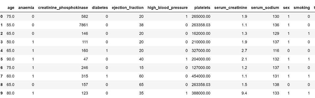
Our purpose is to foretell the DEATH_EVENT binary column on the finish of the DataFrame.

First, let’s standardize our information utilizing StandardScaler. Though not as essential as distance algorithms, information standardization might be very useful in bettering the gradient descent algorithms used through the coaching course of. I wish to scale the whole lot besides the final column (goal).
from sklearn.preprocessing import StandardScaler

scaler = StandardScaler()
heart_failure_data_std = scaler.fit_transform(heart_failure_data.iloc[:,:-1])
Now you can carry out a easy prepare and take a look at break up. We use sklearn to do that and depart 20% of the dataset for testing functions.
X_train, X_test, y_train, y_test = train_test_split(
    heart_failure_data_std, heart_failure_data.DEATH_EVENT, test_size = 0.2, random_state=10
)
You additionally must convert your information to torch.tensor.
X_train = torch.from_numpy(X_train).kind(torch.float)
X_test = torch.from_numpy(X_test).kind(torch.float)
y_train = torch.from_numpy(y_train.values).kind(torch.float)
y_test = torch.from_numpy(y_test.values).kind(torch.float)
As soon as the info is prepared, it is time to match the neural community.
Coaching a Vanilla Linear Neural Community
After you have your information in place, it is time to prepare your first neural community. We’ll use an identical structure as we did within the earlier weblog put up within the sequence, utilizing a linear model of a neural community that may deal with linear patterns.
from torch import nn

class LinearModel(nn.Module):
    def __init__(self):
        tremendous().__init__()
        self.layer_1 = nn.Linear(in_features=12, out_features=5)
        self.layer_2 = nn.Linear(in_features=5, out_features=1)

    def ahead(self, x):
        return self.layer_2(self.layer_1(x))
This neural community makes use of pytorch’s nn.Linearmodule to create a neural community with one deep layer (one enter layer, a deep layer, and an output layer).
You possibly can create your personal class by inheriting nn.Module, however you can even (extra elegantly) do the identical factor utilizing the nn.Sequential constructor.
model_0 = nn.Sequential(
 nn.Linear(in_features=12, out_features=5),
 nn.Linear(in_features=5, out_features=1)
)

good! Subsequently, the neural community comprises a single interior layer with 5 neurons (this may be seen by out_features=5 within the first layer).
This interior layer receives the identical variety of connections from every enter neuron. The in_features of 12 within the first layer replicate the variety of options, and the out_features of 1 within the second layer replicate the output (a single worth between 0 and 1).
Outline a loss operate and optimizer to coach the neural community. Outline BCEWithLogitsLoss (PyTorch 2.1 documentation) as this loss operate (a torch implementation of binary cross entropy, appropriate for classification issues) and because the optimizer we use stochastic gradient descent (utilizing torch.optim.SGD ).
# Binary Cross entropy
loss_fn = nn.BCEWithLogitsLoss()

# Stochastic Gradient Descent for Optimizer
optimizer = torch.optim.SGD(params=model_0.parameters(),
 lr=0.01)
Lastly, we additionally wish to calculate the accuracy for every epoch of the coaching course of, so we design a operate to calculate that.
def compute_accuracy(y_true, y_pred):
    tp_tn = torch.eq(y_true, y_pred).sum().merchandise()
    acc = (tp_tn / len(y_pred)) * 100
    return acc
Time to coach the mannequin! Let’s prepare the mannequin for 1000 epochs and see how a easy linear community can deal with this information.
torch.manual_seed(42)

epochs = 1000

train_acc_ev = []
test_acc_ev = []

# Construct coaching and analysis loop
for epoch in vary(epochs):

    model_0.prepare()

    y_logits = model_0(X_train).squeeze()

    loss = loss_fn(y_logits,
                   y_train)
    # Calculating accuracy utilizing predicted logists
    acc = compute_accuracy(y_true=y_train,
                      y_pred=torch.spherical(torch.sigmoid(y_logits)))

    train_acc_ev.append(acc)

    # Coaching steps
    optimizer.zero_grad()
    loss.backward()
    optimizer.step()
    model_0.eval()

    # Inference mode for prediction on the take a look at information
    with torch.inference_mode():


        test_logits = model_0(X_test).squeeze()
        test_loss = loss_fn(test_logits,
                            y_test)
        test_acc = compute_accuracy(y_true=y_test,
                               y_pred=torch.spherical(torch.sigmoid(test_logits)))
        test_acc_ev.append(test_acc)

    # Print out accuracy and loss each 100 epochs
    if epoch % 100 == 0:
        print(f"Epoch: {epoch}, Loss: {loss:.5f}, Accuracy: {acc:.2f}% | Take a look at loss: {test_loss:.5f}, Take a look at acc: {test_acc:.2f}%")
Sadly, the neural community we simply constructed isn’t ok to unravel this drawback. Let’s check out the evolution of coaching and testing accuracy.
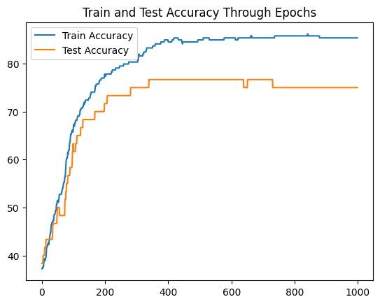
(I am plotting accuracy as an alternative of loss as a result of it is simpler to interpret on this drawback)
Curiously, our neural community isn’t in a position to enhance the accuracy on the take a look at set very a lot.
Utilizing the information gained from earlier weblog posts, you may strive including extra layers and neurons to your neural community. Let’s run each and see the outcomes.
deeper_model = nn.Sequential(
 nn.Linear(in_features=12, out_features=20),
 nn.Linear(in_features=20, out_features=20),
 nn.Linear(in_features=20, out_features=1)
)

Our deeper mannequin is a little more complicated with further layers and extra neurons, however that does not result in improved community efficiency.

Although the mannequin turns into extra complicated, it doesn’t make the classification drawback extra correct.
To have the ability to obtain extra efficiency, it is advisable unlock a brand new characteristic of Neural Networks: the Activation characteristic.
Enter nonlinearity!
Even when making the mannequin wider and bigger does not yield important enhancements, there should be one thing else that may enhance efficiency utilizing neural networks, proper?
That is the place we will use activation features. On this instance, we return to an easier mannequin, however this time with the next twist:
model_non_linear = nn.Sequential(
 nn.Linear(in_features=12, out_features=5),
 nn.ReLU(),
 nn.Linear(in_features=5, out_features=1)
)
What’s the distinction between this mannequin and the primary one? The distinction is that we added a brand new block (nn.ReLU) to the neural community.of Rectifier linear unit is an activation operate that adjustments the calculation of every weight within the neural community.

All values that go via the weights within the neural community are calculated in opposition to this operate. If the product of the characteristic worth and the load is unfavourable, the worth is about to 0, in any other case the calculated worth is assumed. This small change alone provides important energy to the neural community structure. torch has varied activation features that you should utilize, together with nn.ReLU , nn.Tanh , and nn.ELU . Verify this for an outline of all activation features. Link.
For now, there are small tweaks to the neural community structure.
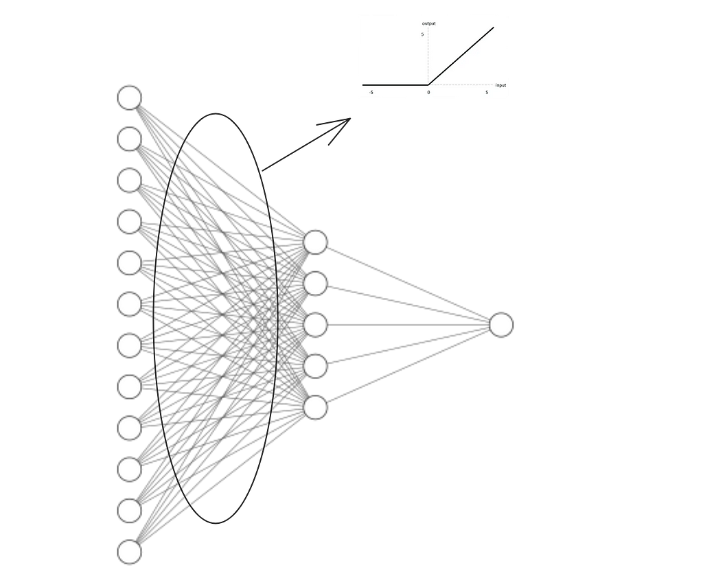
With this little twist within the neural community, all values from the primary layer (represented by nn.Linear(in_features=12, out_features=5)) should go the “ReLU” take a look at.
Let’s take a look at the influence of making use of this structure to our information.
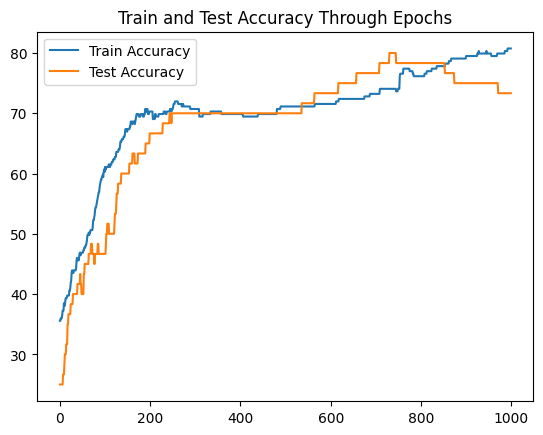
good! Though we will see some efficiency drop after 800 epochs, this mannequin doesn’t exhibit overfitting just like the earlier mannequin. Observe that the dataset could be very small, so randomness alone would possibly enhance the outcomes. Nonetheless, including an activation operate to the Torch mannequin positively has a major influence when it comes to efficiency, coaching, and generalization, particularly when there’s a considerable amount of information to coach on.
Now that the facility of nonlinear activation features, it is essential to know the next:
- You possibly can add activation features to each layer of your neural community.
- The varied activation features embody Different effects on performance and training process.
- torch elegantly offers the power so as to add activation features between layers by leveraging the nn module.
conclusion
Thanks for studying this put up. On this weblog put up, we noticed find out how to incorporate activation features inside the torch neural community paradigm. One other essential idea we perceive is {that a} bigger and extra in depth community doesn’t equate to raised efficiency.
Activation features assist deal with issues which are solved with extra complicated architectures (once more, extra complicated is totally different than greater/broader). These enhance generalization capacity and assist options converge sooner. This is without doubt one of the key options of neural community fashions.
And since it’s broadly utilized in varied neural fashions, torch wins our favor with its cool implementation of assorted features within the nn.Sequential module.
I hope you get pleasure from it. See you within the subsequent PyTorch put up! The primary PyTorch weblog posts might be discovered right here and right here.We extremely suggest you to go to. PyTorch Zero to Master Coursean amazing free useful resource that impressed the methodology behind this put up.
Additionally, I look ahead to seeing you on my newly created YouTube channel. data journey Add content material about information science and machine studying right here.
[The dataset used in this blog post is under licence Creative Commons https://bmcmedinformdecismak.biomedcentral.com/articles/10.1186/s12911-020-1023-5#Sec2]
“PyTorch Introduction — Enter NonLinear Capabilities” was initially revealed on “In the direction of Knowledge Science on Medium” and persons are persevering with the dialog by highlighting and responding to this story.


