


my sequence on Outlier Detection. On this article, we have a look at working with categorical knowledge.
Typically when performing outlier detection with tabular knowledge, we begin by changing the info in order that it’s both completely categorical or completely numeric. There are some exceptions, however for probably the most half that is mandatory: most outlier detection algorithms will assume the info is strictly in a single format or the opposite, and we’ll must get the info into the format the detector expects.
If the detector expects categorical knowledge, the numeric options will should be transformed to a categorical format, which typically means binning them. And if the detector expects numeric knowledge, any categorical options should be numerically encoded. That is the extra frequent state of affairs (the vast majority of outlier detection algorithms assume numeric knowledge), and is what we’ll cowl on this article.
Different articles within the sequence embody: Deep Studying for Outlier Detection on Tabular and Picture Knowledge, Distance Metric Studying for Outlier Detection, An Introduction to Utilizing PCA for Outlier Detection, Interpretable Outlier Detection: Frequent Patterns Outlier Issue (FPOF), and Carry out Outlier Detection Extra Successfully Utilizing Subsets of Options.
This text additionally covers some materials from the e-book Outlier Detection in Python.
Outlier Detectors
Some examples of outlier detection algorithms that assume categorical knowledge embody: Frequent Patterns Outlier Issue (FPOF), Affiliation Guidelines, and Entropy-based strategies. Some that work with numeric knowledge embody: Isolation Forests, Native Outlier Issue (LOF), kth Nearest Neighbors (kNN), and Elliptic Envelope.
For those who’re aware of any outlier detection algorithms, it’s extra possible the numeric algorithms, significantly Isolation Forest and LOF; these are most likely probably the most generally used algorithms. Additional, the entire outlier detection algorithms included in scikit-learn and in PYOD (Python Outlier Detection) assume utterly numeric knowledge.
On the identical time, the nice majority of real-world tabular knowledge is definitely blended (containing each numeric and categorical columns), which implies, it’s quite common when performing outlier detection to want to encode the specific columns.
There’s a cause for this: blended knowledge is harder to carry out outlier detection on. Working with knowledge of only one sort (all categorical or all numeric) does simplify the work of discovering probably the most uncommon gadgets within the knowledge.
And, if we work with numeric knowledge, now we have the additional advantage of with the ability to view the info geometrically: as factors in area. If there are, say, 20 numeric columns in a desk, then every row of the info may be considered as a degree in 20-dimensional area. Not less than, we are able to conceptually think about them in 20-d area — the human thoughts can’t really image this. However we can image 2nd and 3d areas and may extrapolate the final concept: we’re in search of factors which might be bodily very distant from most different factors. For instance, in 2nd, we could have knowledge corresponding to:
Right here, we assume the info has simply two options, known as A and B, each with numeric values. Every row within the knowledge is drawn both as a blue dot or a crimson star, with its location primarily based on the values within the A and B columns. The blue dots point out typical knowledge, and the crimson stars signify a subset of the factors that could possibly be fairly thought-about outliers: some factors on the fringes of the clusters, and the factors exterior the clusters (the info has three important clusters, in addition to some factors exterior these).
That is fairly pure in decrease dimensions. Issues are completely different in excessive dimensions, on account of what’s known as the curse of dimensionality, and we do should be aware of that. However, conceptually, the concept of outliers as comparatively remoted factors in high-dimensional area is pretty easy.
Most numeric outlier detectors work by calculating the distances between every pair of factors, and utilizing these distances to establish the factors which might be most uncommon — the factors which have few factors close to them and which might be distant from most different factors. Although, in observe (for effectivity), the algorithms received’t really calculate each pairwise distance (some may be skipped the place it received’t considerably have an effect on the outlier scores), however in precept, that is what the vast majority of numeric outlier detectors are doing.
We want, then, methods to transform categorical knowledge to a numeric format that helps this effectively; that’s, that makes it significant to calculate distances between rows after encoding the specific values as numbers.
Strategies to encode categorical knowledge
With prediction issues, the commonest encoding strategies possible embody:
- One-hot encoding
- Ordinal encoding
- Goal encoding
With outlier detection, the set of choices is a bit completely different, and the strengths and weaknesses of every are additionally completely different. Out of the three strategies listed right here, actually solely One-hot encoding works effectively for outlier detection. With outlier detection, the simplest are possible:
- One-hot encoding
- Depend encoding
I’ll describe how every works, and why some work higher than others for outlier detection. And I’ll clarify why Depend encoding (which is never used with prediction issues) may be fairly helpful with outlier detection.
I also needs to say, apart from these encoding strategies, there are a number of others that may be helpful for prediction. A wonderful library for encoding strategies is Category Encoders. This can possible cowl any of the strategies you’ll need. Most of the strategies offered, although, corresponding to Goal encoding and CatBoost encoding, require a goal column, which is generally not accessible with outlier detection.
For instance, if we had a desk representing historic details about prospects of a enterprise, there could also be a categorical column for “Final Product Bought” and a goal column known as “Will Churn in subsequent 6 Months”. The “Final Product Bought” column could have the distinct values: “Product A”, “Product B”, and “Product C”. To encode these, we are able to calculate how typically the goal column has worth True for every worth (within the coaching knowledge), presumably encoding these as 0.12, 0.43, 0.02 (which means, when the ‘Final Product Bought’ is Product A, 12% of the time the Goal column is True, and the consumer churns within the subsequent 6 months; equally for Product B (43%) and Product C (2%)).
However with outlier detection, we’re working in a strictly unsupervised atmosphere: there isn’t any floor reality worth for the way outlierish every row is, and so no solution to set a Goal column. We will use solely unsupervised encoding strategies, together with One-hot and Depend encoding.
One-hot encoding
To take a look at One-hot encoding, I’ll begin by describing how it’s achieved, after which will have a look at the way it works with distance calculations. Let’s assume we begin with a desk corresponding to the next:
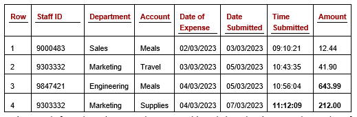 Desk 1: Workers Bills desk
This desk describes employees bills, with one row per expense declare. Assuming we plan to make use of a number of numeric outlier detectors, we’ll must convert the specific columns (Workers ID, Division, and Account) to numbers.
The Date and Time columns can even should be transformed to numeric values. Outlier Detection in Python covers working with date and time knowledge. I don’t have area on this article, however will say rapidly that they are often transformed in quite a few methods. One easy methodology is by calculating the time since some place to begin (known as the epoch). The minimal date or time within the column could also be used, or another date that represents a logical place to begin.
Let’s say we use January 1, 1990. All dates can then be represented because the variety of days since that time. We do, although, additionally want to seize extra details about the dates, such because the day of the week (this can be related, for instance, if employees bills for weekends are uncommon), in the event that they fall on a vacation, and so forth, so we could want to have a look at different encoding strategies as effectively. For this text, although, we’ll focus simply on categorical columns.
If we take into account, for the second, simply the Division column, by One-hot encoding this column, we substitute the column with a sequence of latest columns, one for every distinctive worth within the column. Let’s assume the column had 5 distinct values: Gross sales, Advertising, Engineering, HR, and Communications. We might then have 5 new columns representing these values, corresponding to within the following desk (Desk 2). This reveals simply the Workers ID column, and the brand new columns associated to Division. (The opposite columns can be current as effectively, however are skipped right here for simplicity. An analogous set of columns can be created, for instance, for the Account column).
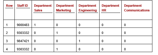 Desk 2: Workers Bills desk with the Division column one-hot encoded (some columns not proven)
Every of the cells within the one-hot Division columns may have a worth of both 0 or 1, indicating if that’s the appropriate worth for this row. We see right here within the first row, an expense declare for Workers 9000483, who’s in Gross sales. On condition that, the column for ‘Division Gross sales’ has a 1 and the opposite columns associated to the Division have a 0. Equally, for one another row: precisely one of many Division columns may have a 1, and all others a 0.
One-hot encoding could be very generally used for outlier detection and generally is a good selection when a characteristic has low cardinality. It will probably, although, break down considerably the place the column has very excessive cardinality. For instance, if the Division column within the authentic employees bills desk had 100 distinct values, it might end in 100 new columns being created, which may create a desk that’s troublesome to work with. I’ll present under, although, that it’s really no worse for distance calculations than with low-cardinality conditions, and so should still be workable.
On the identical time, high-cardinality columns should not typically as helpful for outlier detection as low-cardinality columns. Because of this, we could not wish to embody the Workers Id column within the our outlier detection course of. Although we additionally could: it could nonetheless be informative and helpful to incorporate — for instance, if we want to discover bills which might be giant for that employees, employees which have uncommon numbers of bills, employees which have many comparable bills shut in time and so forth.
One-hot encoding with Isolation Forest
How a lot of an issue producing many further columns depends upon the outlier detection algorithm. Probably the most well-used outlier detection algorithms is Isolation Forest, which doesn’t use distance calculations. As an alternative, it identifies low-density subspaces within the characteristic area and flags the rows that seem in these. Which suggests, it’s nonetheless in search of factors which might be removed from different factors, however does so with out calculating the distances between factors.
I can’t get into the small print of Isolation Forest right here (hopefully a future article, although), however will say rapidly that if a single column is expanded into many columns after encoding (as with One-hot encoding and another encoding schemes), these columns shall be overrepresented within the evaluation of the Isolation Forest algorithm, which we most likely don’t need.
Resulting from some attention-grabbing particulars of how the Isolation Forest algorithm works internally, it’s really often handiest with Isolation Forests to make use of Ordinal encoding. Having stated that, Isolation Forest is without doubt one of the only a few outlier detection algorithms the place that is true — with most different detectors Ordinal encoding works fairly poorly. I’ll describe it under and clarify why that’s the case.
Distance calculations with One-hot encoding
Most numeric outlier detectors, nevertheless, are primarily based on calculating and assessing the distances between factors (or between every level and the info middle, or cluster facilities). This consists of: Native Outlier Issue, k-Nearest Neighbors, Radius, Gaussian Combination Fashions, KDE (Kernel Density Estimation), Elliptic Envelope, One-Class Assist Vector (OCSVM), and quite a few others.
The encoding methodology will have an effect on the distances calculated, and consequently, the outlier scores given to every row. One-hot encoding does often work comparatively effectively with outlier detection for many numeric detectors (together with these primarily based on distance calculations), nevertheless it does have one adverse: as with Isolation Forests, One-hot encoding leads to categorical options being overrepresented in distance calculations, although the impact is much less extreme than with Isolation Forests.
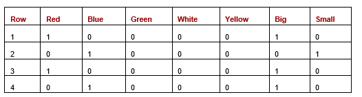
For instance, take into account the next desk (Desk 3), which reveals a dataset with 4 rows and two options. The Color column has 5 values (with two current within the present knowledge) — crimson, blue, inexperienced, white, and yellow. The dimensions column has two values: huge and small.
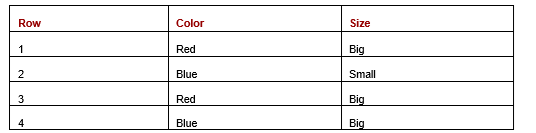 Desk 3: Dataset with Color and Dimension options
The pair-wise distances between the 4 rows are proven within the subsequent desk (Desk 4). There are numerous distance calculations we may use; this methodology leaves the info as categorical (we don’t do any numeric encoding but) and measures the gap between two rows because the variety of values which might be completely different.
As there are two options, a pair of rows can have a distance of zero, one, or two (they’ll have zero, one, or each options completely different). The desk reveals solely the distances between every distinctive pair of rows and reveals every distance solely as soon as (e.g. between Row 1 and Row 2, however between Row 2 and Row 1, which might be the identical; and never between Row 1 and itself), so reveals values solely above the principle diagonal.
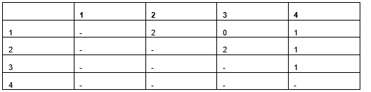 Desk 4: Distances between every pair of rows utilizing a distance metric that considers if options have the identical worth or not.
If we One-hot encode the unique knowledge (from Desk 3), we get:
 Desk 5: Dataset after one-hot encoding
If we calculate the pair-wise distances between the rows utilizing one-hot encoding and both Manhattan or Euclidean distances, now we have the distances proven within the subsequent desk. On this case, as all values are 0 or 1, the Manhattan and Euclidean distances are literally the identical.
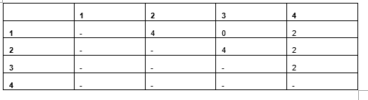 Desk 6: Pairwise Manhattan/Euclidean distances
Utilizing Manhattan (or Euclidean) distance measures, the distances are proportional to when utilizing a rely of the variety of values matching (as we did for Desk 4), however the values are double: when two values within the authentic knowledge mismatch, there shall be two cells within the one-hot encoding mismatched. This isn’t often an issue when working with purely categorical knowledge, nevertheless it does create an undesirable scenario the place now we have blended knowledge.
Take into account Desk 7 with two options: Colour and Weight, the place Weight is numeric.
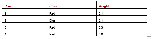 Desk 7: Dataset with one categorical and one numeric characteristic
As soon as one-hot encoded, now we have Desk 8:
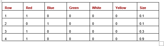 Desk 8: One-hot encoding with one categorical and one numeric characteristic
Right here, once we calculate Euclidean distances between the rows. (We will additionally use Manhattan, Canberra, or some other distance metric, however for this instance, use Euclidean). We present the Euclidean distances within the following desk (Desk 9):
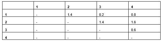 Desk 9: Distances primarily based on Euclidean distances
Rows 1 and a pair of differ within the Color (having the identical weight) and have a Euclidean distance of 1.4. Rows 3 and 4 are completely different in weight (having the identical colour) and have a Euclidean distance of simply 0.6. We will see the distinction in Color is extra vital than Weight in figuring out the gap, although possible it shouldn’t be.
There are two elements that give categorical options extra significance right here than numeric. The primary is that matches versus non-matches have an effect on two one-hot columns, whereas the variations in numeric values have an effect on solely a single column. The second is that distances in binary columns are bigger than in numeric options. Right here, Row 1 and Row 4 have Weight values of 0.1 and 0.9, which have a major distinction of 0.8 — however that is lower than the distinction in two mismatching categorical values, which shall be 2.0 (on condition that two binary columns will mismatch).
An instance working with Manhattan and Euclidean distances is proven within the following itemizing. Within the first case, we create a pair of vectors representing the primary two rows from the earlier knowledge, with 5 one-hot columns for Color and one column for Weight. We then create one other pair of vectors to simulate what it might appear like if the cardinality of Colour had been as a substitute 2, utilizing solely two binary columns.
Right here we present some code testing the Manhattan and Euclidean distances:
from sklearn.metrics.pairwise import euclidean_distances,
manhattan_distances

# Creates knowledge simulating two rows the place 5 binary columns are
# used for one categorical
row_1 = [1, 0, 0, 0, 0, 0.1]
row_2 = [0, 1, 0, 0, 0, 0.1]
print(manhattan_distances([row_1], [row_2]))
print(euclidean_distances([row_1], [row_2]))

# Creates comparable knowledge however with two binary columns for one
# categorical column
row_1 = [1, 0, 0.1]
row_2 = [0, 1, 0.2]
print(manhattan_distances([row_1], [row_2]))
print(euclidean_distances([row_1], [row_2]))
Curiously, in each instances, the 2 rows have a Manhattan distance of two.1 and Euclidean of 1.4: the place we check utilizing solely two binary options for Color as a substitute of 5, the distances are the identical. Equally, growing the cardinality (utilizing greater than 5 binary columns to signify colour) doesn’t have an effect on the gap measures. No matter what number of one-hot columns there are associated to Color, if two rows have the identical color, there shall be 0 variations; and if they’ve completely different colors, there shall be 2 variations (all different columns shall be zero, and due to this fact matching).
So, there may be, as famous, an imbalance between categorical and numeric options, however it’s not made worse by the cardinality of the specific options.
My suggestion, to cut back the over-emphasis in distance calculations, is to switch the 1.0 values within the one-hot columns with 0.25. This can end in rows with completely different values having a complete distinction (with respect to that authentic column) of 0.5 as a substitute of two.0, placing it extra in the identical scale because the numeric options.
Ordinal encoding
Ordinal encoding works by merely giving every distinctive worth in a categorical column a singular quantity. Within the instance above, we could give the values within the Color column values corresponding to:
crimson: 1
blue: 2
inexperienced: 3
white: 4
yellow: 5
So all values of “crimson” would get replaced by 1, and so forth. Equally for the Dimension column: we are able to substitute ‘small” with, say, 1 and “huge” with 2, or with some other numeric values.
As indicated, this does really work effectively for Isolation Forest. Nevertheless it doesn’t are likely to work effectively for many different numeric outlier detectors, together with these primarily based on distances. Ordinal encoding does keep away from creating further columns: every categorical column is translated right into a single numeric column. However, the gap calculations will change into meaningless.
Utilizing the values above, rows with worth yellow can be thought-about 4.0 away from these with worth crimson, whereas these with worth white would solely be 1.0 away from rows with yellow, which make little sense. The distances find yourself utterly arbitrary.
Depend encoding
Depend encoding is definitely way more vital as an encoding approach with outlier detection than with prediction. As with Ordinal encoding, it coverts every categorical column to a single numeric column, however with Depend encoding, does so in a method that the numeric values aren’t random; they’ve which means, and which means that’s related to outlier detection.
Depend encoding additionally produces numeric values which might be easy for distance calculations.
With Depend encoding, the numeric values generated signify the frequency of the worth (uncommon values shall be given small values and customary values giant values), which has some actual data worth when working with outlier detection.
Having a look on the Workers Bills desk, if now we have a distribution of Division values corresponding to:
Gross sales: 1,000
Advertising: 500
Engineering: 100
HR: 10
Communications: 3
Then, these counts would be the encodings. That’s, 1,000 data (these for Gross sales) shall be given worth 1,000; 500 may have worth 500; and so forth. This has the benefit that it could possibly encode values such that uncommon values are usually removed from different values. On this case, the values 10 and three are shut to one another, which implies these 13 data shall be shut to one another, however there are nonetheless solely 13 of them, and they are going to be removed from the opposite 1,600 data. The worth 1,000 is distant from the opposite values, however there are 1,000 data with this encoding, and so these 1000 data are every near 999 others, and would then not be flagged as outliers.
Within the following code, utilizing these values, we generate a easy, single-feature dataset representing the division and create a Native Outlier Issue (LOF) detector to evaluate this. When working with a number of columns, it’s essential to scale any Depend-encoded options to make sure all options are on the identical scale, however as this instance comprises solely a single characteristic, this step could also be skipped. The LOF is ready to appropriately establish the uncommon values as outliers: the 13 uncommon values are given prediction –1 (indicating outliers within the scikit-learn implementation), whereas all others are predicted as 1 (indicating inliers).
import numpy as np
import pandas as pd
from sklearn.neighbors import LocalOutlierFactor

# Creates a dataset with a single categorical column
vals = np.array(['Sales']*1000 + ['Marketing']*500 + ['Engineering']*100 +
['HR']*10 + ['Communications']*3)

# Depend-encode the column
df = pd.DataFrame({"C1": vals})
vc = df['C1'].value_counts()
map = {x:y for x,y in zip(vc.index, vc.values)}
df['Ordinal C1'] = df['C1'].map(map)

# Makes use of LOF to find out the outliers within the column
clf = LocalOutlierFactor(contamination=0.01)
df['LOF Score'] = clf.fit_predict(df[['Ordinal C1']])
One factor to notice about Depend encoding is that it can provide a number of authentic values the identical numeric code in the event that they occur to have the identical rely. For instance, if Gross sales and Advertising each had 1000 rows, they might each be given an encoding of 1000. Or if Gross sales had 1000 and Advertising had 1001, they might be given practically the identical encoding. For many detectors, this isn’t a problem, however once more, Isolation Forest is a bit completely different and it’s higher to have the ability to distinguish values that truly are distinct, which is feasible with Ordinal encoding.
Figuring out the perfect encoding methodology
Which encoding methodology works finest will range primarily based on the dataset, the outlier detection algorithm, and the forms of outliers you want to discover. Sadly, like many issues in knowledge science, there isn’t any definitive reply as to what’s finest; every methodology may be most well-liked at instances. And, in some instances, it could really work finest to make use of completely different encodings for various options.
As is a typical theme with outlier detection, it may be helpful to take an ensemble strategy, the place rows are encoded in a number of methods. The really anomalous rows will stand out as outliers utilizing every encoding methodology, whereas the extra mildly anomalous will presumably stand out simply utilizing one or one other encoding methodology.
Selecting an encoding methodology may be simpler with prediction issues. With prediction issues, we often have a validation set and may merely strive completely different encoding strategies and decide experimentally which works finest. With outlier detection, although, the issues are often utterly unsupervised (once more, there isn’t any goal column as there isn’t any floor reality as to how outlierish every row is). Which suggests it’s harder to judge the encoding strategies used. We will, although, use a way for evaluating outlier detection methods generally known as Doping.
As effectively, the place the outlier detection system runs over time, it could be attainable to gather labeled knowledge and use this to judge completely different preprocessing strategies together with the encoding of the specific columns.
Scaling
If we had been working with knowledge that was utterly numeric to begin with, we wouldn’t must encode any categorical columns, however we might nonetheless must scale the info, at the least with most numeric outlier detectors. Once more, Isolation Forest is without doubt one of the exceptions, however any primarily based on distance calculations do require that every dimension (every characteristic) is on the identical scale. In any other case the distances between factors (or between the factors and cluster facilities, and so forth.) shall be dominated by options that occur to be on bigger scales.
The identical is true for any categorical columns after encoding. Whatever the encoding methodology used, the brand new numeric options could now be on completely different scales than the options that had been already numeric (and the transformed date or time options). And, if completely different encoding strategies are used for various categorical columns, then even these columns could also be on completely different scales as one another.
Scaling these columns makes use of the identical strategies as numeric columns — we simply have to make sure we embody these new columns. The specifics of doing it will hopefully be coated in a future article, however rapidly: we often use both a min-max, sturdy z-scaling, or spline scaling for this.
All pictures had been by the creator
