Accelerating LLM inference with post-training weight and activation utilizing AWQ and GPTQ on Amazon SageMaker AI

Basis fashions (FMs) and huge language fashions (LLMs) have been quickly scaling, usually doubling in parameter depend inside months, resulting in important enhancements in language understanding and generative capabilities. This speedy progress comes with steep prices: inference now requires huge reminiscence capability, high-performance GPUs, and substantial vitality consumption. This development is obvious within the open supply house. In 2023, TII-UAE launched Falcon 180B, the most important open mannequin on the time. Meta surpassed that in 2024 with Llama 3.1, a 405B dense mannequin. As of mid-2025, the most important publicly accessible mannequin is DeepSeek (V3 – Instruct variant, R1 – Reasoning variant), a mix of consultants (MoE) structure with 671 billion complete parameters—of which 37 billion are lively per token. These fashions ship state-of-the-art efficiency throughout a variety of duties, together with multi-modal search, code technology, summarization, concept technology, logical reasoning, and even PhD-level downside fixing. Regardless of their worth, deploying such fashions in real-world purposes stays largely impractical due to their measurement, value, and infrastructure necessities.

We frequently depend on the intelligence of huge fashions for mission-critical purposes corresponding to customer-facing assistants, medical analysis, or enterprise brokers, the place hallucinations can result in severe penalties. Nonetheless, deploying fashions with over 100 billion parameters at scale is technically difficult—these fashions require important GPU assets and reminiscence bandwidth, making it tough to spin up or scale down situations rapidly in response to fluctuating person demand. In consequence, scaling to 1000’s of customers rapidly turns into cost-prohibitive, as a result of the high-performance infrastructure necessities make the return on funding (ROI) tough to justify. Put up-training quantization (PTQ) presents a sensible different; by changing 16- or 32-bit weights and activations into lower-precision 8- or 4-bit integers after coaching, PTQ can shrink mannequin measurement by 2–8 instances, scale back reminiscence bandwidth necessities, and pace up matrix operations, all with out the necessity for retraining, making it appropriate for deploying massive fashions extra effectively. For instance, the bottom DeepSeek-V3 mannequin requires an ml.p5e.48xlarge occasion (with 1128 GB H100 GPU reminiscence) for inference, whereas its quantized variant (QuixiAI/DeepSeek-V3-0324-AWQ) can run on smaller situations corresponding to ml.p5.48xlarge (with 640 GB H100 GPU reminiscence) and even ml.p4de.24xlarge (with 640 GB A100 GPU reminiscence). This effectivity is achieved by making use of low-bit quantization to much less influential weight channels, whereas preserving or rescaling the channels which have the best influence on activation responses, and conserving activations in full precision—dramatically lowering peak reminiscence utilization.

Quantized fashions are made potential by contributions from the developer group—together with tasks like Unsloth AI and QuixiAI (formerly: Cognitive Computations)—that make investments important time and assets into optimizing LLMs for environment friendly inference. These quantized fashions will be seamlessly deployed on Amazon SageMaker AI utilizing just a few traces of code. Amazon SageMaker Inference gives a completely managed service for internet hosting machine studying, deep studying, and huge language or imaginative and prescient fashions at scale in a cheap and production-ready method. On this publish, we discover why quantization issues—the way it permits lower-cost inference, helps deployment on resource-constrained {hardware}, and reduces each the monetary and environmental influence of recent LLMs, whereas preserving most of their authentic efficiency. We additionally take a deep dive into the rules behind PTQ and reveal the best way to quantize the mannequin of your selection and deploy it on Amazon SageMaker.

The steps are:

1. Select mannequin
2. Select W_xA_y method (W_xA_y right here implies weights and activations, which will likely be mentioned in depth later on this publish)
3. Select algorithm (AWQ, GPTQ, SmoothQuant, and so forth)
4. Quantize
5. Deploy and inference

As an instance this workflow and assist visualize the method, we’ve included the next circulate diagram.

Conditions

To run the instance notebooks, you want an AWS account with an AWS Identification and Entry Administration (IAM) function with permissions to handle assets created. For extra data, see Create an AWS account.

If that is your first time working with Amazon SageMaker Studio, you first have to create a SageMaker area.

By default, the mannequin runs in a shared AWS managed digital personal cloud (VPC) with web entry. To reinforce safety and management entry, you must explicitly configure a personal VPC with applicable safety teams and IAM insurance policies primarily based in your necessities.

Amazon SageMaker AI gives enterprise-grade safety features to assist hold your knowledge and purposes safe and personal. We don’t share your knowledge with mannequin suppliers, offering you full management over your knowledge. This is applicable to all fashions—each proprietary and publicly accessible, together with DeepSeek-R1 on SageMaker. For extra data, see Configure safety in Amazon SageMaker AI.

As a finest follow, it’s at all times beneficial to deploy your LLM’s endpoints inside your VPC and behind a personal subnet with out web gateways and ideally with no egress. Ingress from the web also needs to be blocked to reduce safety dangers.

On this publish, we use LiteLLM Python SDK to standardize and summary entry to Amazon SageMaker real-time endpoints and LLMPerf instrument for analysis of efficiency of our quantized fashions. See Set up within the LLMPerf GitHub repo for setup directions.

Weights and activation methods (WₓAᵧ)

As the dimensions of LLMs continues to develop, deploying them effectively turns into much less about uncooked efficiency and extra about discovering the precise steadiness between pace, value, and accuracy. In real-world eventualities, quantization begins with three core concerns:

• The scale of the mannequin you must host
• The associated fee or goal {hardware} accessible for inference
• The suitable trade-off between accuracy and inference pace

Understanding how these components form quantization decisions is essential to creating LLMs viable in manufacturing environments. We’ll discover how post-training quantization methods like AWQ and generative pre-trained transformers quantization (GPTQ) assist navigate these constraints and make state-of-the-art fashions deployable at scale.

Weights and activation: A deep dive

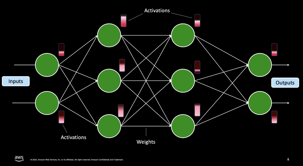
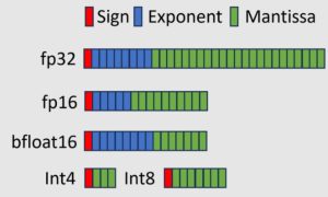
In neural networks, weights are the static, realized parameters saved within the mannequin—consider them because the mounted coefficients that form how inputs are mixed—whereas activations are the dynamic values produced at every layer while you run knowledge by the community, representing the response of every neuron to its inputs. The previous determine illustrates weights and activations in a mannequin circulate. We seize their respective precisions with the shorthand WₓAᵧ, the place Wₓ is the bit-width for weights (for instance, 4-bit or 8-bit) and Aᵧ is the bit-width for activations (for instance, 8-bit or 16-bit). For instance, W4A16 means weights are saved as 4-bit integers (usually with per-channel, symmetric or uneven scaling) whereas activations stay in 16-bit floating level. This notation tells you which ones components of the mannequin are compressed and by how a lot, serving to you steadiness reminiscence use, compute pace, and accuracy.

W4A16 (or W4A16_symmetric)

W4A16 refers to 4-bit precision for weights and 16-bit for activations, utilizing a symmetric quantization for weights. Symmetric quantization means the quantizer’s vary is centered round zero (absolutely the minimal and most of the burden distribution are set to be equal in magnitude). Utilizing 4-bit integer weights yields an 8-times discount in weight reminiscence in comparison with FP32 (or 4 instances in comparison with FP16), which could be very engaging for deployment. Nonetheless, with solely 16 quantization ranges (−8 to +7 for a 4-bit signed integer, in a symmetric scheme), the mannequin is susceptible to quantization error. If the burden distribution isn’t completely zero-centered (for instance, if weights have a slight bias or just a few massive outliers), a symmetric quantizer may waste vary on one facet and never have sufficient decision the place the majority of values lie. Research have discovered {that a} naive 4-bit symmetric quantization of LLM weights can incur a noticeable accuracy drop and is mostly inferior to utilizing an uneven scheme at this low bit-width. The symmetric W4A16 method is especially a baseline; with out further methods (like AWQ’s scaling or GPTQ’s error compensation), 4-bit weight quantization wants cautious dealing with to keep away from severe degradation.

W4A16_asymmetric

Utilizing 4-bit weights with an uneven quantization improves upon the symmetric case by introducing a zero-point offset. Uneven quantization maps the minimal weight to the bottom representable integer and the utmost weight to the very best integer, relatively than forcing the vary to be symmetric round zero. This enables the small 4-bit scale to cowl the precise vary of weight values extra successfully. In follow, 4-bit weight quantization with uneven scaling considerably outperforms the symmetric method when it comes to mannequin accuracy. By higher using all 16 ranges of the quantizer (particularly when the burden distribution has a non-zero imply or outstanding outliers on one facet), the uneven W4A16 scheme can scale back the quantization error. Trendy PTQ strategies for 4-bit LLMs nearly at all times incorporate some type of uneven or per-channel scaling because of this. For instance, one method is group-wise quantization the place every group of weights (for instance, every output channel) will get its personal min-max vary—successfully an uneven quantization per group—which has been recognized as a sweet-spot when mixed with 4-bit weights. W4A16 with uneven quantization is the popular technique for pushing weights to ultra-low precision, as a result of it yields higher perplexity and accuracy retention than a symmetric 4-bit mapping.

W8A8

This denotes absolutely quantizing each weights and activations to 8-bit integers. INT8 quantization is a well-understood, broadly adopted PTQ method that often incurs minimal accuracy loss in lots of networks, as a result of 256 distinct ranges (per quantization vary) are often adequate to seize the wanted precision. For LLMs, weight quantization to 8-bit is comparatively easy—research has shown that replacing 16-bit weights with INT8 usually causes negligible change in perplexity. Activation quantization to 8-bit, nonetheless, is more difficult for transformers due to the presence of outliers—occasional very massive activation values in sure layers. These outliers can power a quantizer to have an especially massive vary, making most values use solely a tiny fraction of the 8-bit ranges (leading to precision loss). To handle this, methods like SmoothQuant redistribute a few of the quantization problem from activations to weights—primarily cutting down outlier activation channels and scaling up the corresponding weight channels (a mathematically equal transformation) in order that activations have a tighter vary that matches effectively in 8 bits. With such calibrations, LLMs will be quantized to W8A8 with little or no efficiency drop. The good thing about W8A8 is that it permits end-to-end integer inference—each weights and activations are integers—which present {hardware} can exploit for quicker matrix multiplication. Absolutely INT8 fashions usually run quicker than blended precision fashions, as a result of they’ll use optimized INT8 arithmetic all through.

W8A16

W8A16 makes use of 8-bit quantization for weights whereas conserving activations in 16-bit precision (usually FP16). It may be seen as a weight-only quantization state of affairs. The reminiscence financial savings from compressing weights to INT8 are important (a 2 instances discount in comparison with FP16, and 4 instances in comparison with FP32) and, as famous, INT8 weights often don’t harm accuracy in LLMs. As a result of activations stay in excessive precision, the mannequin’s computation outcomes are almost as correct as the unique—the primary supply of error is the minor quantization noise in weights. Weight-only INT8 quantization is thus a really secure selection that yields substantial reminiscence discount with nearly no mannequin high quality loss.

Many sensible deployments begin with weight-only INT8 PTQ as a baseline. This method is particularly helpful while you need to scale back mannequin measurement to suit on a tool inside a given reminiscence price range with out doing advanced calibration for activations. When it comes to pace, utilizing INT8 weights reduces reminiscence bandwidth necessities (benefiting memory-bound inference eventualities) and may barely enhance throughput, nonetheless the activations are nonetheless 16-bit, and the compute models may not be absolutely using integer math for accumulation. If the {hardware} converts INT8 weights to 16-bit on the fly to multiply by FP16 activations, the pace achieve could be restricted by that conversion. For memory-bound workloads (frequent with LLMs at small batch sizes), INT8 weights present a noticeable speed-up as a result of the bottleneck is commonly fetching weights from reminiscence. For compute-bound eventualities (corresponding to very massive batch throughput), weight-only quantization alone yields much less profit—in these instances, you could possibly quantize activations (shifting to W8A8) to make use of quick INT8×INT8 matrix multiplication absolutely. In abstract, W8A16 is simple to implement quantization scheme that dramatically cuts mannequin measurement with minimal threat, whereas W8A8 is the subsequent step to maximise inference pace at the price of a extra concerned calibration course of.

Abstract

The next desk gives a high-level overview of the WₓAᵧ paradigm.

Inference acceleration by PTQ methods

As outlined earlier, LLMs with excessive parameter counts are extraordinarily resource-intensive at inference. Within the following sections, we discover how PTQ reduces these necessities, enabling cheaper and performant inference. As an illustration, a Llama 3 70B parameter mannequin at FP16 precision doesn’t match right into a single A100 80 GB GPU and requires no less than two A100 80 GB GPUs for affordable inference at scale, making deployment each pricey and impractical for a lot of use instances. To handle this problem, PTQ converts a educated mannequin’s weights (and typically activations) from high-precision floats (for instance, 16- or 32-bit) to lower-bit integers (for instance, 8-bit or 4-bit) after coaching. This compression can shrink mannequin measurement by 2–8 instances, enabling the mannequin to slot in reminiscence and lowering reminiscence bandwidth calls for, which in flip can pace up inference.

Crucially, PTQ requires no further coaching—in contrast to quantization-aware coaching (QAT), which includes quantization into the fine-tuning course of. PTQ avoids the prohibitive retraining value related to billion-parameter fashions. The problem is to quantize the mannequin rigorously to reduce any drop in accuracy or enhance in perplexity. Trendy PTQ methods attempt to retain mannequin efficiency whereas dramatically bettering deployment effectivity.

Put up-training quantization algorithms

Quantizing a complete mannequin on to 4-bit or 8-bit precision may appear easy, however doing so naïvely usually ends in substantial accuracy degradation—significantly underneath lower-bit configurations. To beat this, specialised PTQ algorithms have been developed that intelligently compress mannequin parameters whereas preserving constancy. On this publish, we concentrate on two broadly adopted and well-researched PTQ methods, every taking a definite method to high-accuracy compression:

• Activation-aware weights quantization (AWQ)
• Generative pre-trained transformers quantization (GPTQ)

Activation conscious weights quantization

AWQ is a PTQ method that targets weight-only quantization at very low bit widths (usually 4-bit) whereas conserving activations in increased precision, corresponding to FP16. The core idea is that not all weights contribute equally to a mannequin’s output; a small subset of salient weights disproportionately influences predictions. By figuring out and preserving roughly 1% of those vital weight channels—these related to the most important activation values—AWQ can dramatically shut the hole between 4-bit quantized fashions and their authentic FP16 counterparts when it comes to perplexity. In contrast to conventional strategies that rank significance primarily based on weight magnitude alone, AWQ makes use of activation distributions to search out which weights really matter. Early outcomes confirmed that leaving the highest 1% of channels in increased precision was sufficient to keep up efficiency—however this introduces {hardware} inefficiencies resulting from mixed-precision execution. To get round this, AWQ introduces a chic workaround of per-channel scaling.

Throughout quantization, AWQ amplifies the weights of activation-salient channels to scale back relative quantization error and folds the inverse scaling into the mannequin, so no specific rescaling is required throughout inference. This adjustment eliminates the overhead of mixed-precision computation whereas conserving inference purely low-bit. Importantly, AWQ achieves this with out retraining—it makes use of a small calibration dataset to estimate activation statistics and derive scaling components analytically. The strategy avoids overfitting to calibration knowledge, making certain robust generalization throughout duties. In follow, AWQ delivers near-FP16 efficiency even at 4-bit precision, displaying far smaller degradation than conventional post-training strategies like RTN (round-to-nearest). Whereas there’s nonetheless a marginal enhance in perplexity in comparison with full-precision fashions, the trade-off is commonly negligible given the three–4 instances discount in reminiscence footprint and bandwidth. This effectivity permits deployment of very massive fashions—as much as 70 billion parameters—on a single high-end GPU corresponding to an A100 or H100. Briefly, AWQ demonstrates that with cautious, activation-aware scaling, precision will be centered the place it issues most, attaining low-bit quantization with minimal influence on mannequin high quality.

Generative pre-trained transformers quantization (GPTQ)

GPTQ is one other PTQ technique that takes an error-compensation-driven method to compressing massive language fashions. GPTQ operates layer by layer, aiming to protect every layer’s output as carefully as potential to that of the unique full-precision mannequin. It follows a grasping, sequential quantization technique: at every step, a single weight or a small group of weights is quantized, whereas the remaining unquantized weights are adjusted to compensate for the error launched. This retains the output of every layer tightly aligned with the unique. The method is knowledgeable by approximate second-order statistics, particularly an approximation of the Hessian matrix, which estimates how delicate the output is to adjustments in every weight. This optimization process is usually known as optimum mind quantization, the place GPTQ rigorously quantizes weights in an order that minimizes cumulative output error.

Regardless of its sophistication, GPTQ stays a one-shot PTQ technique—it doesn’t require retraining or iterative fine-tuning. It makes use of a small calibration dataset to run ahead passes, amassing activation statistics and estimating Hessians, however avoids any weight updates past the grasping compensation logic. The result’s an impressively environment friendly compression method: GPTQ can quantize fashions to three–4 bits per weight with minimal accuracy loss, even for large fashions. For instance, the strategy demonstrated compressing a 175 billion-parameter GPT mannequin to three–4 bits in underneath 4 GPU-hours, with negligible enhance in perplexity, enabling single-GPU inference for the primary time at this scale. Whereas GPTQ delivers excessive accuracy, its reliance on calibration knowledge has led some researchers to notice gentle overfitting results, particularly for out-of-distribution inputs. Nonetheless, GPTQ has turn out to be a go-to baseline in LLM quantization due to its robust steadiness of constancy and effectivity, aided by mathematical optimizations corresponding to quick Cholesky-based Hessian updates that make it sensible even for fashions with tens or a whole lot of billions of parameters.

Utilizing Amazon SageMaker AI for inference optimization and mannequin quantization

On this part, we cowl the best way to implement quantization utilizing Amazon SageMaker AI. We stroll by a codebase that you should use to rapidly quantize a mannequin utilizing both the GPTQ or AWQ technique on SageMaker coaching jobs backed by a number of GPU situations. The code makes use of the open supply vllm-project/llm-compressor bundle to quantize dense LLM weights from FP32 to INT4.

All code for this course of is out there within the amazon-sagemaker-generativeai GitHub repository. The llm-compressor venture gives a streamlined library for mannequin optimization. It helps a number of algorithms—GPTQ, AWQ, and SmoothQuant—for changing full- or half-precision fashions into lower-precision codecs. Quantization takes place in three steps, described within the following sections. The complete implementation is out there in post_training_sagemaker_quantizer.py, with arguments supplied for easy execution.

Step 1: Load mannequin utilizing HuggingFace transformers

Load the mannequin weights with out attaching them to an accelerator. The llm-compressor library robotically detects accessible {hardware} and offloads weights to the accelerator as wanted. As a result of it performs quantization layer by layer, your entire mannequin doesn’t want to slot in accelerator reminiscence without delay.

def quantize_model(
    args: argparse.Namespace
) -> None:
    strive:

        ...
        # load mannequin
        mannequin = AutoModelForCausalLM.from_pretrained(
            args.model_id,
            torch_dtype="auto",
            device_map=None,
            trust_remote_code=True
        )
        # load tokenizer
        tokenizer_or_processor = AutoTokenizer.from_pretrained(
            args.model_id,
            trust_remote_code=True
        )
       ...

Step 2: Choose and cargo the calibration dataset

A calibration dataset is used throughout PTQ to estimate activation ranges and statistical distributions in a pretrained LLM with out retraining. Instruments like llm-compressor use this small, consultant dataset to run ahead passes and acquire statistics corresponding to minimal and most values or percentiles. These statistics information the quantization of weights and activations to scale back precision whereas preserving mannequin accuracy. You should utilize any tokenized dataset that displays the mannequin’s anticipated enter distribution for calibration.

from llmcompressor import oneshot
from llmcompressor.modifiers.awq import AWQModifier
from llmcompressor.modifiers.quantization import GPTQModifier
....

def preprocess_data(
    dataset: Any,
    tokenizer: AutoTokenizer,
    max_sequence_length: int
) -> Any:
    def preprocess(instance):
        return {
            "textual content": tokenizer.apply_chat_template(
                instance["messages"],
                tokenize=False,
            )
        }

    def tokenize(pattern: Dict) -> Dict:
        return tokenizer(
            pattern["text"],
            padding=False,
            max_length=max_sequence_length,
            truncation=True,
            add_special_tokens=False,
        )

    dataset = dataset.map(preprocess)
    dataset = dataset.map(tokenize,  remove_columns=dataset.column_names)
    return dataset

Step 3: Run PTQ on the candidate mannequin

The oneshot technique in llm-compressor performs a single-pass (no iterative retraining) PTQ utilizing a specified recipe, making use of each weight and activation quantization (and optionally sparsity) in a single cross.

• num_calibration_samples defines what number of enter sequences (for instance, 512) are used to simulate mannequin conduct, gathering the activation statistics essential for calibrating quantization ranges.
• max_seq_length units the utmost token size (for instance, 2048) for these calibration samples, so activations mirror the worst-case sequence context, making certain quantization stays correct throughout enter lengths.

Collectively, these hyperparameters management the representativeness and protection of calibration, straight impacting quantization constancy.

The modifier courses (GPTQModifier, AWQModifier) settle for a schema parameter that defines the bit-width for each weights and activations. By means of this parameter, you possibly can specify codecs corresponding to W8A8 (8-bit weights and activations) or W4A16 (4-bit weights with 16-bit activations), providing you with fine-grained management over precision trade-offs throughout mannequin layers.

        ...
        ... 
        logger.information(f"Configuring {args.algorithm.higher()} quantization")
        if args.algorithm == "awq":

            quant_scheme = args.awq_quantization_scheme
            recipe = [
                AWQModifier(
                    ignore=[val.rstrip() for val in args.ignore_layers.split(',')],
                    scheme=args.awq_quantization_scheme,
                    targets=[val.rstrip() for val in args.include_targets.split(',')]
                )
            ]

        ...
        elif args.algorithm == "gptq":

            quant_scheme = args.gptq_quantization_scheme
            recipe = [
                GPTQModifier(
                    ignore=[val.rstrip() for val in args.ignore_layers.split(',')],
                    scheme=args.gptq_quantization_scheme,
                    targets=[val.rstrip() for val in args.include_targets.split(',')]
                )
            ]
       ...
       ...
        oneshot(
            mannequin=mannequin,
            dataset=processed_dataset,
            recipe=recipe,
            max_seq_length=args.max_sequence_length, # <- Set max sequence size
            num_calibration_samples=args.num_calibration_samples, # <- Set max calibration - variety of iterations of stats calculation
            output_dir=save_dir,
            trust_remote_code_model=True
        )

Structure sample for quantization on Amazon SageMaker AI

All the workflow, proven within the following determine, is carried out within the post_training_sagemaker_quantizer.py script and will be executed as a SageMaker coaching job on an occasion with NVIDIA GPU assist (corresponding to ml.g5.2xlarge) for accelerated quantization.

This course of doesn’t contain coaching or fine-tuning the mannequin. The coaching job is used solely to run PTQ with GPU acceleration.

...
hyperparameters = {
    'model-id': 'meta-llama/Llama-3.1-8B-Instruct',
    'dataset-id': 'HuggingFaceH4/ultrachat_200k',
    'dataset-split': 'train_sft',
    'dataset-seed': 42,
    'algorithm': 'gptq',
    'max-sequence-length': 1024,
    'num-calibration-samples': 256,
    'ignore-layers': 'lm_head',
    'include-targets': 'Linear',
    'gptq-quantization-scheme': 'W8A8',
}

quantization_estimator = PyTorch(
    entry_point="post_training_sagemaker_quantizer.py",
    source_dir="./scripts",
    instance_type="ml.g6e.2xlarge",
    instance_count=1,
    function=function,
    framework_version='2.4.0',
    py_version='py311',
    hyperparameters=hyperparameters,
    surroundings={"HF_TOKEN": "my-awesome-hf-token"}
)
...

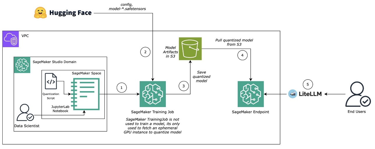
After a mannequin is quantized, it is going to be saved to Amazon Easy Storage Service (Amazon S3) straight as an output from the SageMaker coaching job. We’ll uncompress the mannequin and host it as a SageMaker real-time endpoint utilizing a Amazon SageMaker AI massive mannequin inference (LMI) container, powered by vLLM. To search out the newest photos, see AWS Deep Learning Framework Support Policy for LMI containers (see SageMaker section).

...

prebaked_inference_image_uri = f"763104351884.dkr.ecr.{sagemaker.Session().boto_session.region_name}.amazonaws.com/djl-inference:0.33.0-lmi15.0.0-cu128"
...
quant_model = sagemaker.Mannequin(
    image_uri=prebaked_inference_image_uri,
    env={
        "HF_MODEL_ID": f"{remote_upload_s3uri}/", <- Your mannequin S3 path
        "OPTION_MAX_MODEL_LEN": "12000",
        "OPTION_GPU_MEMORY_UTILIZATION": "0.95",
        "OPTION_ENABLE_STREAMING": "false",
        "OPTION_ROLLING_BATCH": "auto",
        "OPTION_MODEL_LOADING_TIMEOUT": "3600",
        "OPTION_PAGED_ATTENTION": "false",
        "OPTION_DTYPE": "fp16",
    },
    function=function,
    title=model_name,
    sagemaker_session=sagemaker.Session()
)
...
pretrained_predictor = quant_model.deploy(
    endpoint_name=endpoint_name,
    initial_instance_count=1,
    instance_type="ml.g5.2xlarge",
    container_startup_health_check_timeout=600,
    wait=False
)
print(f"Your Endpoint: {endpoint_name} is now deployed!")
```

You now have a SageMaker real-time endpoint serving your quantized mannequin and prepared for inference. You possibly can question it utilizing the SageMaker Python SDK or litellm, relying in your integration wants.

 from litellm import completion

response = completion(
        mannequin=f"sagemaker/{endpoint_name}", 
        messages=[{ "content": "Hello", "role": "user"}, { "content": "You are a helpful assistant that follows instructions", "role": "system"}],
        temperature=0.1,
        max_tokens=64
    )

Mannequin efficiency

We are going to use an ml.g5.2xlarge occasion for Llama-3.1-8B and Qwen-2.5-VL-7B fashions and ml.p4d.24xlarge occasion for Llama-3.1-70B mannequin and an LMI container v15 with vLLM backend as a serving framework.

The next is a code snippet from the deployment configuration:

lmi_env = {
    "SERVING_FAIL_FAST": "true",
    "OPTION_ASYNC_MODE": "true",
    "OPTION_ROLLING_BATCH": "disable",
    "OPTION_MAX_MODEL_LEN": "8192",
    "OPTION_TENSOR_PARALLEL_DEGREE": "max",
    "OPTION_ENTRYPOINT": "djl_python.lmi_vllm.vllm_async_service",
}

This efficiency analysis’s main aim is to point out the relative efficiency of mannequin variations on totally different {hardware}. The mixtures aren’t absolutely optimized and shouldn’t be seen as peak mannequin efficiency on an occasion kind. At all times make certain to check utilizing your knowledge, site visitors, and I/O sequence size. The next is efficiency benchmark script:

#!/bin/bash
export LLM_PERF_CONCURRENT=1
export LLM_PERF_MAX_REQUESTS=$(expr $LLM_PERF_CONCURRENT * 10)
export LLM_PERF_SCRIPT_DIR=$HOME/5_projects/llmperf

export LLM_PERF_OUTPUT=outputs/test-2025-07-08-21-45-57-221

mkdir -p $LLM_PERF_OUTPUT
cp "$0" "${LLM_PERF_OUTPUT}"/

python3 ${LLM_PERF_SCRIPT_DIR}/token_benchmark_ray.py 
    --model "sagemaker/model-2025-07-08-21-01-10-147" 
    --mean-input-tokens 512 
    --stddev-input-tokens 32 
    --mean-output-tokens 256 
    --stddev-output-tokens 16 
    --max-num-completed-requests ${LLM_PERF_MAX_REQUESTS} 
    --timeout 1800 
    --num-concurrent-requests ${LLM_PERF_CONCURRENT} 
    --results-dir "${LLM_PERF_OUTPUT}" 
    --llm-api litellm 
    --additional-sampling-params '{}'

Efficiency metrics

To know the influence of PTQ optimization methods, we concentrate on 5 key inference efficiency metrics—every providing a unique lens on system effectivity and person expertise:

• GPU reminiscence utilization: Signifies the proportion of complete GPU reminiscence actively used throughout inference. Greater reminiscence utilization suggests extra of the mannequin or enter knowledge is loaded into GPU reminiscence, which might enhance throughput—however extreme utilization may result in reminiscence bottlenecks or out-of-memory errors.
• Finish-to-end latency: Measures the whole time taken from enter submission to last output. That is vital for purposes the place responsiveness is essential, corresponding to real-time programs or user-facing interfaces.
• Time to first token (TTFT): Captures the delay between enter submission and the technology of the primary token. Decrease TTFT is particularly necessary for streaming or interactive workloads, the place perceived responsiveness issues greater than complete latency.
• Inter-token latency (ITL): Tracks the common time between successive token outputs. A decrease ITL ends in smoother, faster-seeming responses, significantly in long-form textual content technology.
• Throughput: Measures the variety of tokens generated per second throughout all concurrent requests. Greater throughput signifies higher system effectivity and scalability, enabling quicker processing of huge workloads or extra simultaneous person periods.

Collectively, these metrics present a holistic view of inference conduct—balancing uncooked effectivity with real-world usability. Within the subsequent sections of this publish, we consider three candidate fashions—every various in measurement and structure—to validate inference efficiency metrics after quantization utilizing AWQ and GPTQ algorithms throughout totally different WₓAᵧ methods. The chosen fashions embrace:

• Llama-3.1-8B-Instruct: An 8-billion parameter dense decoder-only transformer mannequin optimized for instruction following. Revealed by Meta, it belongs to the LLaMA (Massive Language Mannequin Meta AI) household and is well-suited for general-purpose pure language processing (NLP) duties.
• Llama-3.3-70B-Instruct: A 70-billion parameter mannequin additionally from Meta’s LLaMA collection, this bigger variant presents considerably improved reasoning and factual grounding capabilities, making it best for high-performance enterprise use instances.
• Qwen2.5-VL-7B-Instruct: A 7-billion parameter vision-language mannequin developed by Alibaba’s Institute for Clever Computing. It helps each textual content and picture inputs, combining a transformer-based textual content spine with a visible encoder, making it appropriate for multimodal purposes.

Be aware that every mannequin was examined on a unique occasion kind: Llama-3.1-8B on ml.g5.2xlarge, Llama-3.3-70B on ml.p4dn.24xlarge, and Qwen2.5-VL-7B on ml.g6e.4xlarge.

GPU reminiscence utilization

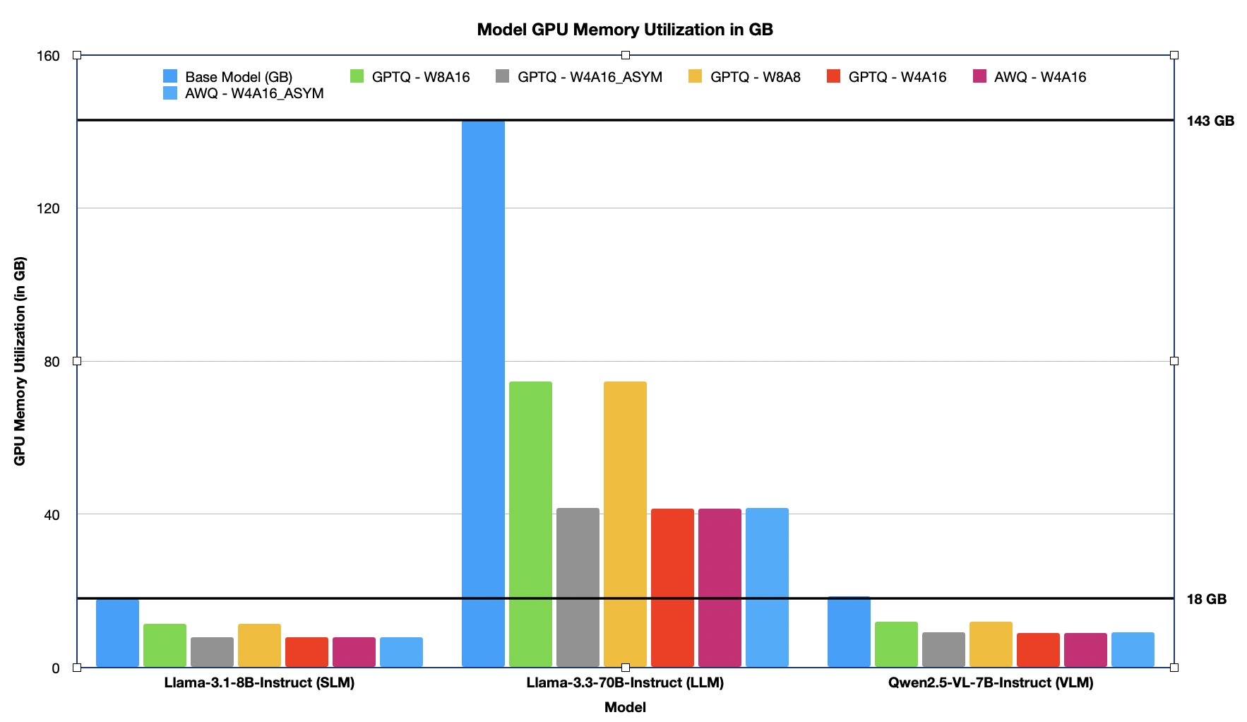
GPU reminiscence utilization displays how a lot gadget reminiscence is consumed throughout mannequin execution and straight impacts deployability, batch measurement, and {hardware} choice. Decrease reminiscence utilization permits working bigger fashions on smaller GPUs or serving extra concurrent requests on the identical {hardware}. Quantization improves compute effectivity and considerably reduces the reminiscence footprint of LLMs. By changing high-precision weights (for instance, FP16 or FP32) into lower-bit codecs corresponding to INT8 or FP8, each AWQ and GPTQ methods allow fashions to eat considerably much less GPU reminiscence throughout inference. That is vital for deploying massive fashions on memory-constrained {hardware} or rising batch sizes for increased throughput. Within the following desk and chart, we listing and visualize the GPU reminiscence utilization (in GB) throughout the fashions underneath a number of quantization configurations. The proportion discount is in contrast in opposition to the bottom (unquantized) mannequin measurement, highlighting the reminiscence financial savings achieved with every WₓAᵧ technique, which ranges from ~30%–70% much less GPU reminiscence utilization after PTQ.

The determine beneath illustrates the GPU reminiscence footprint (in GB) of the mannequin in its uncooked (unquantized) type in comparison with its quantized variants. Quantization ends in ~30%–70% discount in GPU reminiscence consumption, considerably reducing the general reminiscence footprint.

Finish-to-end latency

Finish-to-end latency measures the whole time taken from the second a immediate is obtained to the supply of the ultimate output token. It’s a vital metric for evaluating user-perceived responsiveness and general system efficiency, particularly in real-time or interactive purposes.

Within the following desk, we report end-to-end latency in seconds throughout various concurrency ranges (C=1 to C=128) for three fashions of various measurement and modality (Llama-3.1-8B, Llama-3.3-70B, and Qwen2.5-VL-7B) underneath totally different quantization methods.

The next graphs displaying finish to finish latency for various concurrency ranges for various fashions.

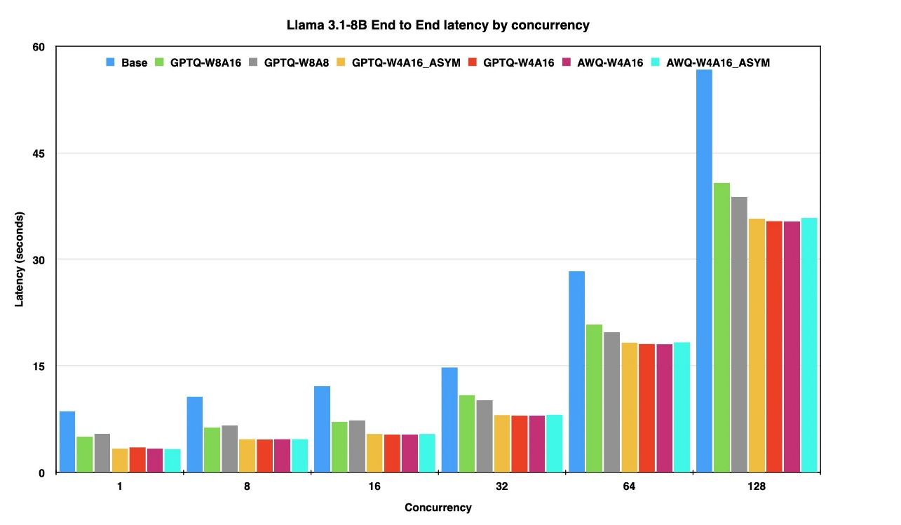
The determine above presents the end-to-end latency of the Llama 3-8B mannequin in its uncooked (unquantized) type and its quantized variants throughout concurrency ranges starting from 1 to 128 on the identical occasion.

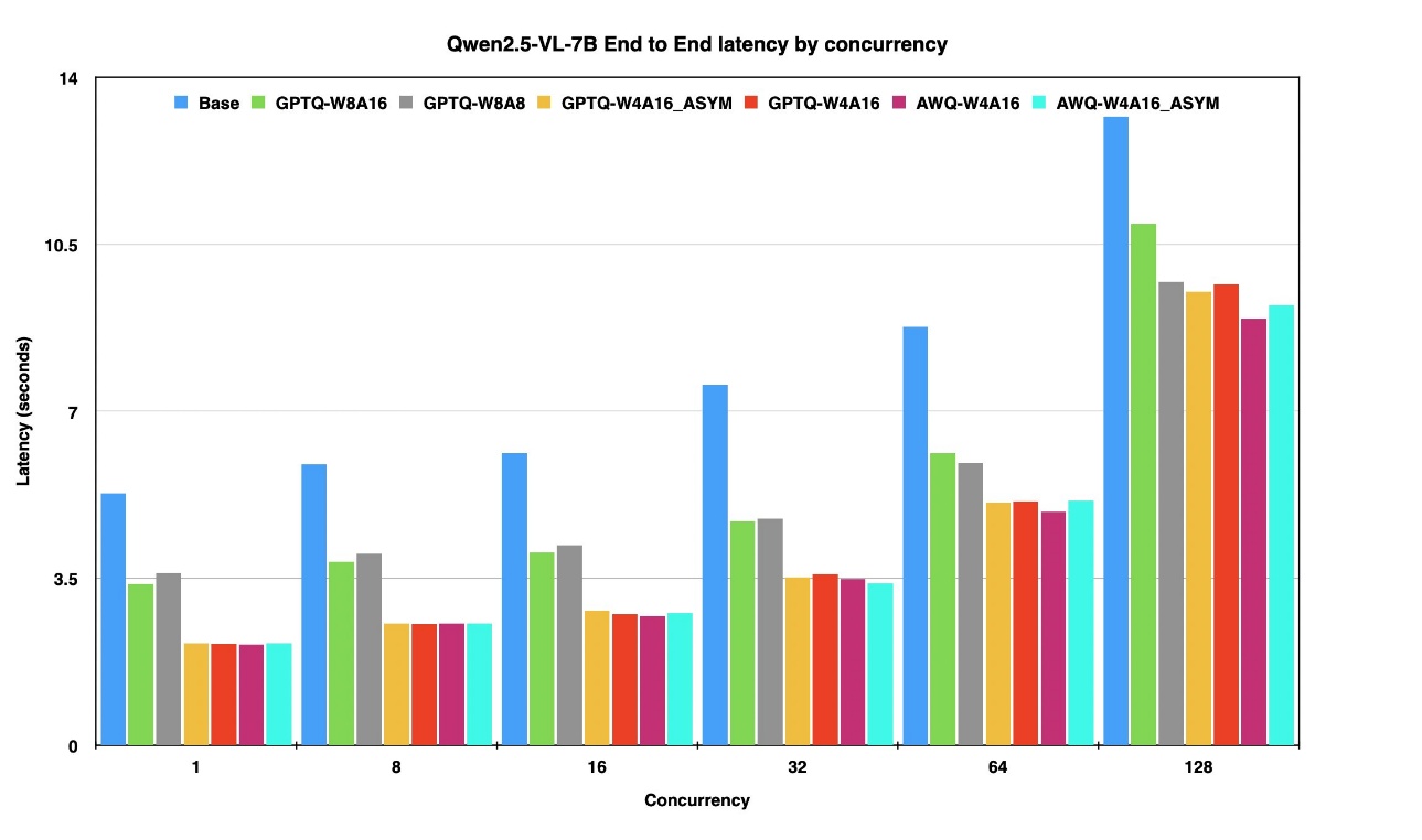
The determine above presents the end-to-end latency of the Qwen 2.7-7B mannequin in its uncooked (unquantized) type and its quantized variants throughout concurrency ranges starting from 1 to 128 on the identical occasion.

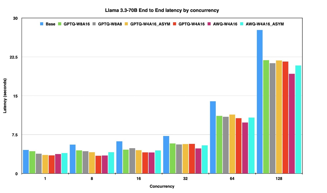
The determine above presents the end-to-end latency of the Llama 3-70B mannequin in its uncooked (unquantized) type and its quantized variants throughout concurrency ranges starting from 1 to 128 on the identical occasion.

Time to first token

TTFT measures the delay between immediate submission and the technology of the primary token. This metric performs an important function in shaping perceived responsiveness—particularly in chat-based, streaming, or interactive purposes the place preliminary suggestions time is vital. Within the following desk, we examine TTFT in seconds for 3 fashions of various measurement and modality—Llama-3.1-8B, Llama-3.3-70B, and Qwen2.5-VL-7B—underneath totally different quantization methods. As concurrency will increase (from C=1 to C=128), the outcomes spotlight how quantization methods like AWQ and GPTQ assist keep low startup latency, making certain a smoother and quicker expertise even underneath excessive load.

Inter-token latency

ITL measures the common time delay between the technology of successive tokens. It straight impacts the smoothness and pace of streamed outputs—significantly necessary in purposes involving long-form textual content technology or voice synthesis, the place delays between phrases or sentences can degrade person expertise. Within the following desk, we analyze ITL in seconds throughout three fashions of various measurement and modality—Llama-3.1-8B, Llama-3.3-70B, and Qwen2.5-VL-7B—underneath totally different quantization schemes. As concurrency scales up, the outcomes illustrate how quantization methods like AWQ and GPTQ assist keep low per-token latency, making certain fluid technology even underneath excessive parallel hundreds.

Throughput

Throughput measures the variety of tokens generated per second and is a key indicator of how effectively a mannequin can scale underneath load. Greater throughput straight permits quicker batch processing and helps extra concurrent person periods. Within the following desk, we current throughput outcomes for Llama-3.1-8B, Llama-3.3-70B, and Qwen2.5-VL-7B throughout various concurrency ranges and quantization methods. Quantized fashions keep—and in lots of instances enhance—throughput, because of diminished reminiscence bandwidth and compute necessities. The substantial reminiscence financial savings from quantization permits a number of mannequin employees to be deployed on a single GPU, significantly on high-memory situations. This multi-worker setup additional amplifies complete system throughput at increased concurrency ranges, making quantization a extremely efficient technique for maximizing utilization in manufacturing environments.

Conclusion

Put up-training quantization (PTQ) methods like AWQ and GPTQ have confirmed to be efficient options for deploying basis fashions in manufacturing environments. Our complete testing throughout totally different mannequin sizes and architectures demonstrates that PTQ considerably reduces GPU reminiscence utilization. The advantages are evident throughout all key metrics, with quantized fashions displaying higher throughput and diminished latency in inference time, together with high-concurrency eventualities. These enhancements translate to diminished infrastructure prices, improved person expertise by quicker response instances, and the pliability of deploying bigger fashions on resource-constrained {hardware}. As language fashions proceed to develop in scale and complexity, PTQ presents a dependable method for balancing efficiency necessities with infrastructure constraints, offering a transparent path to environment friendly, cost-effective AI deployment.

On this publish, we demonstrated the best way to streamline LLM quantization utilizing Amazon SageMaker AI and the llm-compressor module. The method of changing a full-precision mannequin to its quantized variant requires only a few easy steps, making it accessible and scalable for manufacturing deployments. By utilizing the managed infrastructure of Amazon SageMaker AI, organizations can seamlessly implement and serve quantized fashions for real-time inference, simplifying the journey from improvement to manufacturing. To discover these quantization methods additional, confer with our GitHub repository.

Particular because of everybody who contributed to this text: Giuseppe Zappia, Dan Ferguson, Frank McQuillan and Kareem Syed-Mohammed.

Concerning the authors

Pranav Murthy is a Senior Generative AI Information Scientist at AWS, specializing in serving to organizations innovate with Generative AI, Deep Studying, and Machine Studying on Amazon SageMaker AI. Over the previous 10+ years, he has developed and scaled superior laptop imaginative and prescient (CV) and pure language processing (NLP) fashions to sort out high-impact issues—from optimizing international provide chains to enabling real-time video analytics and multilingual search. When he’s not constructing AI options, Pranav enjoys taking part in strategic video games like chess, touring to find new cultures, and mentoring aspiring AI practitioners. Yow will discover Pranav on LinkedIn

Dmitry Soldatkin is a Senior AI/ML Options Architect at Amazon Internet Providers (AWS), serving to prospects design and construct AI/ML options. Dmitry’s work covers a variety of ML use instances, with a main curiosity in Generative AI, deep studying, and scaling ML throughout the enterprise. He has helped corporations in lots of industries, together with insurance coverage, monetary providers, utilities, and telecommunications. You possibly can join with Dmitry on LinkedIn.